A Forensic Investigation to Unravel Climate Model Biases in Teleconnections

By: Dr. Xiaocen Shen

Teleconnections are usually manifested as recurring patterns which link weather and climate anomalies (departures from long-term average) over large distances across the globe (e.g., Wallace and Gutzler 1981). Therefore, they play an important role in shaping climate variability and regional climate change. One striking example is El Niño-Southern Oscillation (ENSO) teleconnection (Figure 1). ENSO is the most prominent year-to-year internal variability in the climate system, although ENSO itself occurs in the tropical Pacific and is reflected as a fluctuation between unusually warm and cold conditions, it excites wave-trains propagating into the extratropics which then strongly affect the precipitation and temperature over mid-high latitudes (e.g., Trenberth et al. 1998). Moreover, the extratropical circulation response to ENSO can further influence the upward propagation of planetary waves in the midlatitudes, thereby leading to significant changes of the stratospheric polar vortex (SPV) via the wave-mean flow interaction (e.g. Domeisen et al., 2019). The induced SPV anomaly, in return, can further descend into the troposphere, modulating the weather condition in the midlatitudes. For instance, this ENSO-SPV linkage is shown to strongly contribute to the cooling over northern Europe in late winter following El Niño (e.g., Ineson and Scaife 2009). Hence, studying teleconnections is not only helpful to better understand the atmospheric circulation variability, but is also key to improving the prediction skill. 

Figure 1. Schematic of ENSO teleconnections (from Domeisen et al. 2019)

While the observations are the starting point for studying teleconnections, the limited records make it difficult to draw robust conclusions based on observations alone. On the one hand, the climate system is complex, and the relationships sometimes vary in different time periods (e.g., Dong and McPhaden 2017). On the other hand, the simple correlation between two circulations does not always indicate a physical teleconnection, it can sometimes instead reflect co-varying changes in response to other factors (Kretschmer et al. 2021).  

To address this problem, climate model simulations are widely used as they can provide more samples. However, climate models do not always agree with the observed teleconnections, in which case the discrepancy is known as model bias.. There are two main potential reasons for the discrepancy. First, the climate models may fail to capture the key physical processes and therefore cannot reproduce the teleconnections. Second, due to the limited sample size in the observations, the discrepancy may reflect the internal variability of the climate system. Therefore, to confidently use models to study teleconnections and the related aspects, scientific judgement is needed to justify the suitability of models when there are apparent discrepancies (e.g. Jain et al. 2023). In our recent research, we have advocated the use of a forensic investigation approach to understand the discrepancies between climate models and observations, which then helps to make the decision on whether the model outputs can be trusted.  

The literal definition of a forensic investigation is the scientific analysis of physical evidence from a crime scene. The logic behind it is to conduct a thorough examination of the evidence to establish the facts and uncover the truth. In the context of assessing model discrepancies in teleconnections, a physically-based analysis is required to understand their origin, which can then provide an evidential basis for deciding whether a model is appropriate for a given scientific purpose. Since the logic is similar with that of solving crime puzzles, the term forensic is used here to characterize our approach (Figure 12). In the following, the case of ENSO-SPV relationship will be shown as an example of how to extract reliable information from the model output using the forensic investigation approach.

Figure 2. The logic of forensic investigation to unravel the climate model biases (adapted from images by Freepik)

In a climate model called the MIROC6, the ENSO-SPV relationship is opposite to observations. At the first glance, it seems that this model is not suitable for studying the ENSO-SPV relationship and related scientific questions. However, according to the physically-based analysis, we found that MIROC6 model actually well captures the relevant dynamical processes, including the extratropical response to ENSO, the anomalous upward propagation of planetary waves, and the wave-mean flow interaction in the stratosphere. The discrepancy is further shown to be mainly related to the wave propagation within the stratosphere, which eventually lead to the different SPV response. This reflects that the causal linkage between ENSO and SPV is shaped by other factors and/or background states, known as the state dependence. Therefore, although the model shows an opposite ENSO-SPV relationship to the observation, it is physically reasonable.  

Furthermore, the observations show a state dependence similar to that of the model results, in that the observed ENSO-SPV relationship is not stable and is shaped by other factors, such as the ocean background condition (e.g. Rao et al. 2019). The observational evidence neither supports nor contradicts this state dependence found in the model due to the limited sample size. Thus, depending on the specific purpose of the research, different choices can be made in how to use the model simulations.  

If the study does not require a stable teleconnection, for example, if it is used to study non-stationarity and state dependence, then the model can be used directly to provide conditional information. On the other hand, if the study requires a stable teleconnection consistent with observations, then the model should be used only after the application of a physically-based bias adjustment. In the ENSO-SPV relationship case, under the assumption that the state-dependance is spurious, a physically-based bias adjustment is applied to SPV, which effectively aligns the modelled ENSO-SPV relationship with the observations, thereby removes the model-observations discrepancy in the surface air temperature response. 

This case gives an example of how the forensic approach could help us to better understand the difference between models and observations, allowing us to make full use of climate model outputs (Figure 3). Similar physically-based approaches have been widely used in the climate research in recent decades (e.g., Kretschmer et al. 2020; Shepherd 2021), providing us with more opportunities to gain a more holistic view of model performance and to extract more information from models 

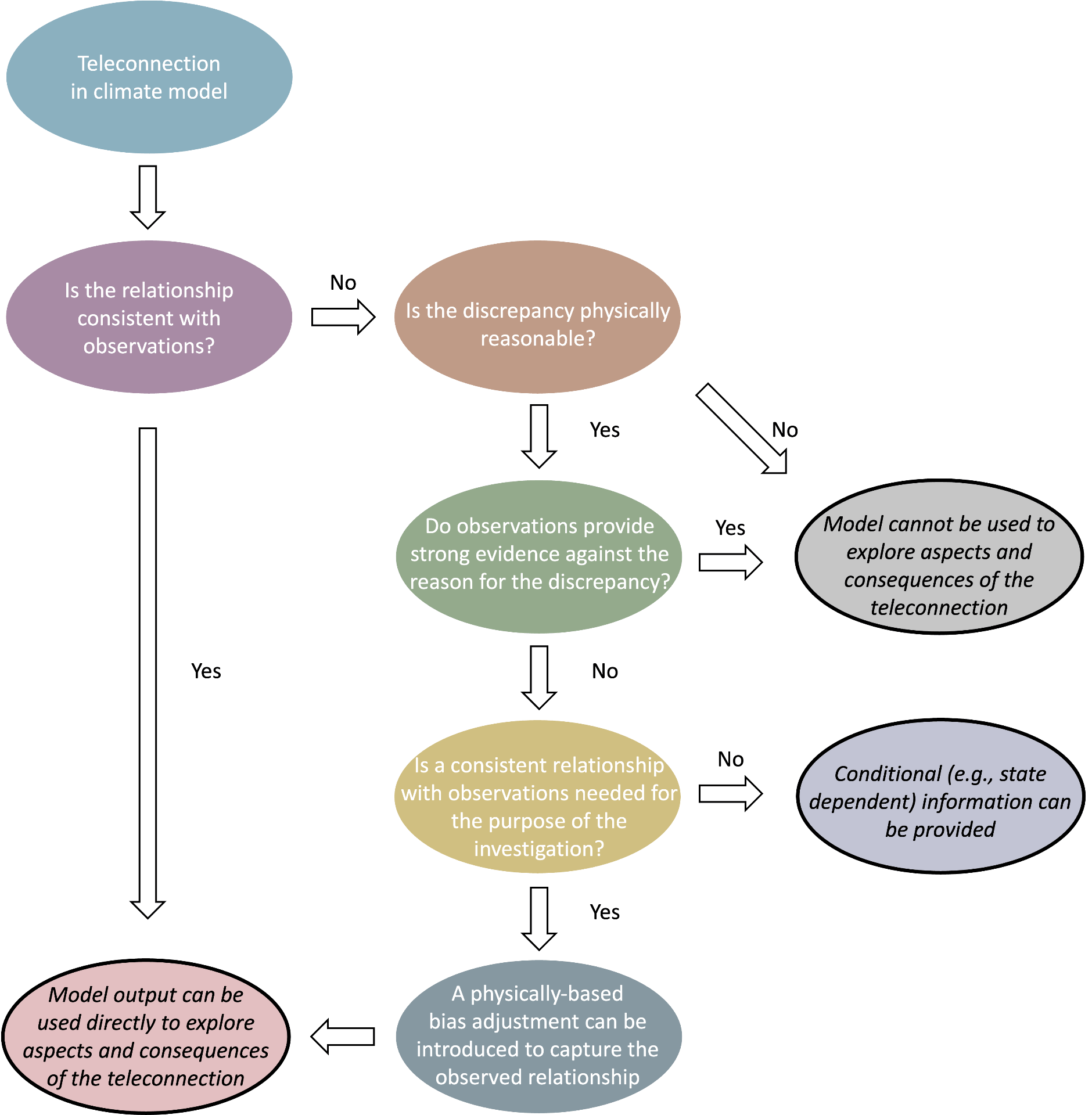
Figure 3. The forensic investigation processes. The direction of the arrows indicates the order in which actions are taken. The bubbles enclosed by the black contours indicate the conclusions about whether we can trust the model and how to use the model outputs.

Further Reading/References: 

Domeisen, D. I. V., Garfinkel, C. I., & Butler, A. H. (2019). The teleconnection of El Nino South-ern Oscillation to the stratosphere. Reviews of Geophysics, 57(1), 5-47. https://doi.org/10.1029/2018rg000596 

Dong, L., & McPhaden, M. J. (2017). Why has the relationship between Indian and Pacific ocean decadal variability changed in recent decades? Journal of Climate, 30(6), 1971-1983. https://doi.org/10.1175/jcli-d-16-0313.1 

Ineson, S., & Scaife, A. A. (2009). The role of the stratosphere in the European climate response to El Nino. Nature Geoscience, 2(1), 32-36. https://doi.org/10.1038/ngeo381 

Jain, S., Scaife, A. A., Shepherd, T. G., Deser, C., Dunstone, N., Schmidt, G. A., Trenberth, K. E., & Turkington, T. (2023). Importance of internal variability for climate model assessment. npj Cli-mate and Atmospheric Science, 6(1), 68. https://doi.org/10.1038/s41612-023-00389-0 

Kretschmer, M., Adams, S. V., Arribas, A., Prudden, R., Robinson, N., Saggioro, E., & Shepherd, T. G. (2021). Quantifying causal pathways of teleconnections. Bulletin of the American Meteorological Society, 102(12), E2247-E2263. https://doi.org/10.1175/bams-d-20-0117.1 

Kretschmer, M., Zappa, G., & Shepherd, T. G. (2020). The role of Barents–Kara sea ice loss in projected polar vortex changes. Weather Climate Dynamics, 1(2), 715-730. https://doi.org/10.5194/wcd-1-715-2020 

Rao, J., Garfinkel, C. I., & Ren, R. C. (2019). Modulation of the Northern winter stratospheric El Nino-Southern Oscillation teleconnection by the PDO. Journal of Climate, 32(18), 5761-5783. https://doi.org/10.1175/jcli-d-19-0087.1 

Shepherd, T. G. (2021). Bringing physical reasoning into statistical practice in climate-change sci-ence. Climatic Change, 169(1-2), 2. https://doi.org/10.1007/s10584-021-03226-6 

Trenberth, K. E., Branstator, G. W., Karoly, D., Kumar, A., Lau, N. C., & Ropelewski, C. (1998). Progress during TOGA in understanding and modeling global teleconnections associated with tropical sea surface temperatures. Journal of Geophysical Research-Oceans, 103(C7), 14291-14324. https://doi.org/10.1029/97jc01444 

Wallace, J. M., & Gutzler, D. S. (1981). Teleconections in the geopotential height field during the Northern Hemisphere winter. Monthly Weather Review, 109(4), 784-812. https://doi.org/10.1175/1520-0493(1981)109<0784:Titghf>2.0.Co;2 


Posted in Climate | Leave a comment

Ground-based radar systems for environmental monitoring

By: Dr. Veronica Escobar-Ruiz

RADAR is the acronym for RAdio Detention And Ranging, it is a process in which an electromagnetic wave is transmitted through an antenna and in the presence of an object this radio wave bounces towards a receiving antenna. The reflected magnitude and phase of the signal depend on the characteristics of the object (e.g. size, shape, orientation, and material). Radar frequencies are classified in bands by the Institute of Electrical and Electronics Engineers (IEEE) depending on their range on the electromagnetic spectrum such as L-, S-, C-, X- and Xu-Band which ranges are 1-2GHz, 2-4GHz, 4-8GHz, 8-12Ghz and 12-18GHz, respectively. 

One of the most common radar techniques is the Synthetic Aperture Radar (SAR) which creates 2D images, like photograph in optical systems. SAR systems on satellite platforms has become an important data acquisition method known as remote sensing. In satellite data, the smaller available spatial resolution is 5m xa 20m but usually averaged to 20m x 20m for easier interpretation. However, this coarse resolution limits the ability of airspace systems to differentiate features in the scanning area (e.g., soil, vegetation, water bodies). Hence, the use of ground radar systems can provide high-resolution data reducing this spatial uncertainty. 

In the Meteorology Department at the University of Reading, we have developed a pair of ground-radar systems, a UAV-Radar and a Radar-Rig, which operate at a C-band frequency range using a Frequency Modulated Continuous Wave (FMCW). The radar under the FMCW method transmits a radio wave which changes linearly over a wide range of frequencies providing a better range resolution compared with unmodulated systems. 

The UAV-Radar consists of a C-band system, an array of path-antennas, and a small single-board computer (Figure 1a). The radar operates a frequency range from 5.2 GHz to 6.0 GHz, using one transmitter and two receiver antennas. The construction of a mechanical structure, known as gimbal, provides a movement of the antennas along the vertical direction in degrees and across the horizontal direction for a side-looking or down-looking antenna setting. Additionally, the antennas can be rotated, offering a configuration of different polarisation modes (VV, HH and VH). Similarly, the Radar Rig is a software-controlled instrument running radar from a starting to an ending point on a 3m rail (Figure 1b). The instrument comprises a motor unit, a Vector Network Analyser (VNA) and two horn antennas, one transmitter and one receiver. The software allows different VNA configurations (e.g., frequency range [4GHz to 8GHz], and power) as well as the setting of the motor unit (e.g., start position, scan length and increments). Antennas can be moved vertically along the track in degrees and rotated to provide different polarisation modes. The configuration flexibility of both systems allows a variety of imaging modes such as Real-Beam mapping, Synthetic SAR, SAR Interferometry, 3D tomography and Tomographic Profiling (TP, Morrison and Bennett 2014). The different polarisation modes provide information about the structure of the scanned area. For example, VV mode is sensitive to bare soil and water, whereas VH is to vegetation canopy (leaves and branches).  

Figure 1. a) UAV-Radar system consists of C-band radar, patch antennas, and a single-board computer.

Figure 1. a) UAV-Radar system consists of C-band radar, patch antennas, and a single-board computer.

Figure 1. b) Radar-Rig consists of C-band radar, horn antennas, and a motor unit.

Figure 1. b) Radar-Rig consists of C-band radar, horn antennas, and a motor unit.

The TP method is an analogue to SAR, with the difference of the antennas rotated 90° looking along the track direction. This method allows for vertical backscatter canopy profiles. Both systems have been tested under the TP approach. The UAV-radar system has a high-resolution mapping approximately of 0.5 m along the flight path and 0.5 m vertically (Figure 2), whereas a smaller resolution is achieved with the Radar-Rig (0.22 cm along-track direction, and 3.75 cm vertically, Figure 3). 

Figure 2. Tomography profiling image with reconstruction angle of 0° degrees. Path length of 140 m over trees, gaps in the images correspond to a re-setting time of radar. The top figure is co-polarisation (HH) and the bottom is cross-polarisation (VH). Data was collected in the Stoflaket wetland in northeast Sweden.

Figure 2. Tomography profiling image with reconstruction angle of 0° degrees. Path length of 140 m over trees, gaps in the images correspond to a re-setting time of radar. The top figure is co-polarisation (HH) and the bottom is cross-polarisation (VH). Data was collected in the Stoflaket wetland in northeast Sweden.

Although similar platforms exist (Schartel et al. 2018; Charvat, Kempell, and Coleman 2008), the ones developed at the Meteorology Department (University of Reading) are the first of their kind for environmental monitoring applications (e.g. soil moisture, biomass density, etc). The images obtained in a field by these two ground radar systems can be upscaled to interpreted what the satellite imagery are really “seen”. The results will help to understand how the backscatter signal arises spatially and temporally, the issues that can complicate its interpretation and factors that can contribute to signal distortion. This will allow a more complete and timely exploitation of satellite data. 

Figure 3. (a) Tomography profiling image with projected angle 0°. Path length of 3m over a dwarf shrub. The top figure (a) is co-polarisation (VV).

Figure 3. (a) Tomography profiling image with projected angle 0°. Path length of 3m over a dwarf shrub. This top figure (a) is co-polarisation (VV). Data was collected in the Stoflaket wetland in northeast Sweden.

Figure 3. (b) Tomography profiling image with projected angle 0°. Path length of 3m over a dwarf shrub. This bottom figure (b) is cross-polarisation (VH). Data was collected in the Stoflaket wetland in northeast Sweden.

References and Further Reading:

Charvat, Gregory, Leo Kempell, and Chris Coleman. 2008. “A Low-Power High-Sensitivity X-Band Rail SAR Imaging System [Measurement’s Corner].”  IEEE Antennas and Propagation Magazine 50 (3):108-15. doi: 10.1109/map.2008.4563576. 

Morrison, Keith, and John Bennett. 2014. “Tomographic Profiling—A Technique for Multi-Incidence-Angle Retrieval of the Vertical SAR Backscattering Profiles of Biogeophysical Targets.”  IEEE Transactions on Geoscience and Remote Sensing 52 (2):1350-5. doi: 10.1109/tgrs.2013.2250508. 

Schartel, Markus, Ralf Burr, Winfried Mayer, Nando Docci, and Christian Waldschmidt. 2018. “UAV-Based Ground Penetrating Synthetic Aperture Radar.” In 2018 IEEE MTT-S International Conference on Microwaves for Intelligent Mobility (ICMIM), 1-4. 

Posted in Climate | Leave a comment

Weathering the storm, or even just a blustery day.

By: Dr. Natalie Harvey

Maintaining positive mental well-being fosters resilience, enabling individuals to navigate life’s challenges with clarity, strength, and resilience. It helps us form meaningful relationships and achieve our full potential. Neglecting our mental health can negatively impact all aspects of our lives, impacting not only us as individuals but also the community around us. 

To help create an atmosphere of understanding and compassion within the Department of Meteorology and the wider School of Mathematical, Physical and Computational Sciences we have several initiatives. 

Mental health first aiders 

The School now has a group of colleagues who have trained to be Mental Health First Aiders (MHFA). Their role is to be a point of contact for a colleague who is experiencing a mental health issue or emotional distress. Mental Health First Aiders are not trained to be therapists or psychiatrists, but they can offer initial support through non-judgemental listening and guidance.

For contact information for the MHFAs please see the signs around the School buildings.  

Panel event on Tuesday 14th May 3.30-4.30pm (GU01, Brian Hoskins Building) 

This event will bring together members from across our school community to share their individual insights and experiences. We hope this will encourage people to talk more freely about mental health, reducing stigma and creating a more positive culture within the school. We will also highlight sources of information and guidance for students and staff. All staff and PhD students welcome!  

Useful links: 

https://www.samaritans.org/ – 24 hour, 7 day a week support, whatever you are going through. 

NHS Mental Health Crisis Team: https://www.berkshirehealthcare.nhs.uk/contact-us/i-need-help-now/  

University of Reading Employee Assistance Programme: https://www.reading.ac.uk/human-resources/working-life/health-and-wellbeing/employee-assistance-programme-eap  

Student support line: https://www.reading.ac.uk/essentials/Support-And-Wellbeing/support-line  

Posted in Climate | Leave a comment

What are equatorial waves and how are they linked to heavy rainfall in Southeast Asia?

By: Dr. Samantha Ferrett

What is an equatorial wave and why do we care about them?

Atmospheric equatorial waves are confined to, and move, or propagate, along the equator. Equatorial waves can cause variations in pressure, temperature and winds. Each wave type has a different structure. An idealised example structure of a wave type, called the Kelvin wave, is shown in Figure 1. The arrows show the anomaly of wind associated with the wave, in other words how much the overall wind would change as the wave occurs. In this case Kelvin waves can increase zonal winds or decrease zonal winds. And between those two states can increase the convergence of zonal winds or increase the divergence of zonal winds. This wave propagates eastwards so a given region may experience increased eastward winds, then decreased zonal convergence (where winds are directed away from a particular point, red shading in Figure 1), then decreased eastward winds, and so on, as a wave forms and propagates along the equator. These changes to local atmospheric circulations can have an impact on weather in the regions the wave propagates over. 

Idealised structure of the Kelvin wave. Arrows show horizontal wind anomaly; coloured contours show where anomalous winds are converging (blue) and diverging (red).

In this post I will focus on equatorial wave influences on rainfall in Southeast (SE) Asia, highlighting some of the work that has been done at the University of Reading in the Equatorial waves and FORSEA projects, funded by the Weather and Climate Science for Service Partnership Programme (WCSSP) for SE Asia. SE Asia experiences extreme weather that is notoriously hard to predict, such as heavy rainfall that causes flooding and landslides. Given its location on and around the equator many parts of SE Asia are very susceptible to modulations of local circulation by equatorial waves.  

How are equatorial waves related to heavy rainfall in SE Asia?

In FORSEA and related projects a method has been developed to identify equatorial waves in real world data and forecasts (Yang et al., 2021) which can be used to examine the relationship between equatorial waves and heavy rainfall. In Figure 2 the link between equatorial wave occurrence and heavy rainfall probability is shown. Each panel shows a particular part of a wave occurring over a particular region during a certain season. So, for example, panel a) shows the change in the likelihood of heavy rainfall when there is Kelvin wave convergence over Sumatra in boreal winter (DJF). The yellow shading indicates that heavy rainfall is around three times as likely to occur, orange is four times as likely, and red is five times as likely. The purple lines show the location where winds associated with the Kelvin wave converge. It is clear there is a link between the Kelvin wave wind convergence and an increase of heavy rainfall in Sumatra in DJF, particularly along the coasts.  

There are also many other regions where rainfall increases are linked to equatorial wave occurrences. Another wave type is shown in panel d of Figure 2. This is a different wave type called the n=1 Rossby (R1) wave. This wave propagates westward, unlike the Kelvin wave, and is defined by clockwise and anticlockwise circulation either side of the equator. The solid purple lines in this panel indicate this anticlockwise circulation. This can be linked to phenomena such as tropical storms. When anticlockwise circulation (or “positive vorticity”) related to this wave occurs over Peninsular Malaysia there is again an increase in the likelihood of heavy rainfall over the region. The other panels of Figure 2 demonstrate several other cases. For more details readers can find the full study published in QJRMS (Ferrett et al., 2020). 

This figure taken from ​Ferrett et al. (2020)​. Likelihood of heavy rainfall during days with strong wave activity at low atmospheric level (850hPa). Cases shown are (a) Kelvin wave wind convergence at 100–105°E in DJF, (b) Kelvin wave at 110–115°E in DJF, (c) Kelvin wave at 120–125◦E in DJF, (d) R1 wave at 100–105◦E in DJF, (e) Westward-moving Mixed Rossby Gravity (WMRG) wave convergence in north hemisphere at 100–105°E in DJF, and (f) WMRG wave convergence in south hemisphere at 100–105°E during JJA. A value of 5% and white shading shows no difference from the climatology. Lines show the average convergence (Kelvin and WMRG) or vorticity (R1) on those days with intervals of 5 and 1*10−7s−1 respectively. Solid purple lines indicate convergence/positive vorticity (a measure of anticlockwise circulation), dashed purple lines indicate divergence/negative vorticity.

Why is this useful?

While all this is very interesting, someone may ask, “and what’s the point of this, aside from interest?”. Well, as I mentioned in the introduction our current forecast models can struggle to forecast rainfall in SE Asia. However, the equatorial waves can sometimes be predicted more accurately than the connected rainfall. This means that we can use the forecast of the equatorial waves, and our knowledge of the link between equatorial waves and heavy rainfall likelihood, to create what we have termed a “hybrid dynamical-statistical forecast” of rainfall. In the hybrid forecast we only use the forecast of wave activity, NOT the forecast of the rainfall, to determine how likely heavy rainfall is. This type of forecast has compared favourably to the forecasts of rainfall probability taken directly from the model (Ferrett et al., 2023; Wolf et al., 2023). Furthermore, combining the influence of multiple waves into one hybrid forecast further improves the hybrid forecast skill.  

There is still a lot to learn about how waves and other modes of variability on differing time scales can interact with one another, and what this means for heavy rainfall and other extreme weather events. Ongoing work in our new project FORWARDS is aiming to tackle these questions. 

References

Ferrett, S., Methven, J., Woolnough, S. J., Yang, G. Y., Holloway, C. E., & Wolf, G. (2023). Hybrid Dynamical–Statistical Forecasts of the Risk of Rainfall in Southeast Asia Dependent on Equatorial Waves. Monthly Weather Review, 151(8), 2139–2152. https://doi.org/10.1175/MWR-D-22-0300.1 

Ferrett, S., Yang, G., Woolnough, S. J., Methven, J., Hodges, K., & Holloway, C. E. (2020). Linking extreme precipitation in Southeast Asia to equatorial waves. Quarterly Journal of the Royal Meteorological Society, 146(727), 665–684. https://doi.org/10.1002/qj.3699 

Wolf, G., Ferrett, S., Methven, J., Frame, T. H. A., Holloway, C. E., Martinez-Alvarado, O., & Woolnough, S. J. (2023). Comparison of probabilistic forecasts of extreme precipitation for a global and convection-permitting ensemble and hybrid statistical–dynamical method based on equatorial wave information. Quarterly Journal of the Royal Meteorological Society. https://doi.org/10.1002/QJ.4627 

Yang, G. Y., Ferrett, S., Woolnough, S., Methven, J., & Holloway, C. (2021). Real-Time Identification of Equatorial Waves and Evaluation of Waves in Global Forecasts. Weather and Forecasting, 36(1), 171–193. https://doi.org/10.1175/WAF-D-20-0144.1 

Posted in Climate, Equatorial waves | Leave a comment

Unlocking the secrets of the thunderstorm: what are Thunderstorm Ground Enhancements?

By: Dr. Hripsime Mkrtchyan

Thunderstorm Ground Enhancement is an atmospheric phenomenon which describes a significant increase of the ground-level radiation during thunderstorm activity. This effect is primarily attributed to the acceleration of charged particles by strong electric fields within thunderclouds, which can lead to enhanced gamma radiation detectable at the Earth’s surface.  

In the 1920s, Wilson introduced the theory that the dipole structure of thunderclouds could accelerate electrons toward the ground. However, this theory did not gain immediate acceptance. It was eventually validated about 60 years later, confirming that the electrical configuration of thunderclouds indeed has the capability to accelerate particles downward or upward. 

Over the past decade, the majority of Thunderstorm Ground Enhancements (TGEs) have been detected at the Alikhanyan National Science Laboratory Cosmic Ray Division on Mt. Aragats, Armenia. Equipment which is installed at the station includes particle detectors with different energy thresholds, electric field mills, a lightning detection network, and weather stations. 

Aragats Research Station of Cosmic Ray Division, A. Alikhanyan National Science Lab on mt Aragats (3200 m a.s.l) (copyrights Andranik Keshishyan)

TGEs are more frequently registered in May as the thunderstorm activity is very high in Armenia during that period. TGEs can include high-energy electrons, gamma rays, and neutrons, with durations ranging from a few minutes to several hours depending on the energy level of the particles involved. The flux of the lower-energy particles (less than 3 MeV) can last more than two hours, and  enhancements with high-energy particles (with energies up to 40 MeV) from 1 to 10 min (Chilingarian, 2018). So, thunderclouds can act as natural accelerators, producing particle flux enhancements registered on the ground during thunderstorms.  

The electric field during which particle enhancements are detected on the surface, can have either a positive or negative polarity. These enhancements are attributed to the microphysical processes involving cloud and precipitation particles within these storms. However, the reasons behind the polarity assignment have remained unclear until recently. 

Illustration of full tripole structure for deep (and colder) convection with “negative” Thunderstorm Ground Enhancements (TGE) (right side), and bottom heavy tripole for shallow (and warmer) convection with “positive” TGE (left side). Source Williams E et al 2022 (https://agupubs.onlinelibrary.wiley.com/doi/10.1029/2021JD035957)

In a recent study by Williams et al. (2022), high-energy particle, electric-field, and radar observations have been combined and revealed new insights for these high-energy phenomena. Within the study they used altitude-resolved S-band radar observations of graupel (graupel is a form of precipitation, created through a process called riming) to highlight distinct differences in the structure of storms associated with “positive” and “negative” TGEs on Mount Aragats in Armenia. Their findings indicate that shallow stages of convection are associated with “positive” TGEs, while deep stages of convection are linked to “negative” TGEs. These results align with the temperature-dependent electric tripole structure of thunderclouds. 

The study of Thunderstorm Ground Enhancement is important for advancing our fundamental understanding of atmospheric physics. It can also have practical implications in areas such as aviation safety, radio communication, and environmental monitoring. Future research is expected to delve deeper into the mechanisms behind TGE, exploring how varying atmospheric conditions and storm structures influence ground-level radiation enhancements, to measure vertical profiles of electric fields in TGEs,  also to answer a question if there are storms which are not generating TGEs? Currently, the ongoing research in thunderstorm phenomena and related atmospheric processes continues to shed light on the complex interactions within thunderclouds and their ground-level effects. As technology and methodologies advance, we anticipate more detailed insights that will further unravel the mysteries of Thunderstorm Ground Enhancement. 

In conclusion, TGEs represent a significant interaction between thunderstorm activity and ground-level radiation, highlighting the complex dynamics within thunderclouds and their capability to influence environmental radiation levels. Further research in this area continues to unravel the mechanisms behind TGEs and their implications for understanding atmospheric physics and environmental monitoring. 

References: 

  • Williams E, Mailyan B, Karapetyan G, Mkrtchyan H. Conditions for energetic electrons and gamma rays in thunderstorm ground enhancements,  Journal of Geophysical Research: Atmospheres, 2023 
  • Williams, E., Mkrtchyan, H., Mailyan, B., Karapetyan, G., & Hovakimyan, S. Radar Diagnosis of the Thundercloud Electron Accelerator. Journal of Geophysical Research: Atmospheres, 2022 
  • Chilingarian A., Hovsepyan G., Karapetyan T., Karapetyan G., Kozliner L., Mkrtchyan H., et al. Structure of thunderstorm ground enhancements. Phys. Rev. D 101, 122004, 22 June, 2020  
  • Chilingarian A., Mkrtchyan H. et al. Catalog of 2017 Thunderstorm Ground Enhancement (TGE) events observed on Aragats. Scientific Reports, Vol. 9, Article number: 6253, 2019  
  • Chilingarian, A. (2018). Long lasting low energy thunderstorm ground enhancements and possible Rn-222 daughter isotopes contamination. Physical Review D.
Posted in Climate | Leave a comment

Shedding some light on DARC (the Data Assimilation Research Centre)

By: Dr. Ross Bannister

Data assimilation as a scientific tool for weather forecasting and beyond

In the early 2000s few academic groups around the world were doing research into the activity that we call “data assimilation”. Data assimilation is the process of combining imperfect model information and imperfect observations. This is extremely important for weather forecasting as without accurate and balanced starting conditions, forecast models cannot make meaningful predictions. Indeed all models need to know about “today’s weather” so they can propagate this up-to-the-minute information into a prediction of “tomorrow’s weather”, and beyond.

Knowing today’s weather is non-trivial. The atmosphere is an extensive fluid of around 5 billion cubic km and is described by multiple quantities (wind, temperature, pressure, humidity, cloud, etc.). It is turbulent and chaotic, especially when viewed at small scales. Despite the large number of observations, including from satellite, only a very small part of the volume is measured. This is why data assimilation is needed to combine the ‘theoretical’ model information with the real-world observations.

Data assimilation methods pioneered for weather forecasting are used for other systems too. These include the ocean, the hydrological cycle (e.g. for flood prediction), the carbon cycle, space weather, marine bio-chemical systems, and even disease spread (e.g. Covid). Furthermore, data assimilation is not just used to aid prediction. It is also used to produce datasets of these environmental systems for scientific analysis and societal/commercial exploitation.

Enter the DARC

DARC (the Data Assimilation Research Centre) started in the early 2000s under the directorship of Alan O’Neill, having its HQ in the Meteorology Department at the University of Reading (see the photo of the plaque on display there). It also involved scientists based in Oxford, Cambridge and Edinburgh Universities, and the Rutherford Appleton Laboratory. The initial focus was to use data assimilation to gain information about the stratosphere – a broad, stable layer of the atmosphere above the `weather’, accommodating the ozone layer.

Along with other centres around the UK, DARC was initiated with a budget and the prestigious status as a NERC (Natural Environmental Research Council) Centre of Excellence. Its initial remit was to progress the work of the DARE project (Data Assimilation in Readiness for EnviSat).

DARC scientists worked closely with the Met Office, using its brand new variational data assimilation system, to assimilate data from the EnviSat satellite. EnviSat was launched with great fanfare in 2002 and hosted instruments that could monitor important environmental quantities. DARC was concerned with assimilating stratospheric ozone, temperature and water vapour data from EnviSat (and other) instruments. Stratospheric water vapour, for instance, had never been assimilated before. In September 2002, the stratospheric polar vortex over the south pole – along with the ozone hole – split into two. Such a split in the southern hemisphere had never been seen before. EnviSat, and DARC, saw it happen.

There was also much interest in developing data assimilation methods (such as the variational method mentioned above). Early projects included the development of methods to extract the maximum amount of information from satellite observations, and using physical principles to better quantify errors in the models that observations are meant to reduce.

DARC has been led by several people, who have each encouraged DARC to grow in different directions. In the mid 2000s Martin Ehrendorfer became the director, then Peter Jan van Leeuwen, and then Alberto Carrassi. Since 2021 DARC has been led jointly between Sarah Dance and Amos Lawless. The DARC logo has changed over the years (see below).

Its status – as a NERC funded Centre of Excellence – remained until about 2008, when much of its remit was officially absorbed into NCEO (the National Centre for Earth Observation). DARC, however, remains as the identity of an active research group at the University of Reading.

DARC today

Some DARC members at the 2023 Christmas meal.

DARC is currently made up of about 25 scientists. Many still work on weather-related problems, but others work on a wider range of environmental systems, such as those mentioned above.

The variational method (much developed from the early days) is still the workhorse of weather forecasting, but DARC’s research also embraces ensemble, particle, and hybrid methods of solving theoretical and practical assimilation problems. DARC also runs an annual training course.

Incidentally, all of these data assimilation methods emerge from a fundamental theorem of probability called Bayes’ Theorem (reflecting the inevitable probabilistic approaches of dealing with uncertainty in complex systems), which DARC’s work has been faithful to from the very beginning.

This blog entry first appeared on the DARC blog site. You can read more about DARC and their work through their excellent blogs at: https://research.reading.ac.uk/met-darc/news-and-events/darc-blogs/

Posted in Climate | Leave a comment

The evolution and destruction of Saturn’s rings

By: Dr. James O’Donoghue

Saturn, thanks to its system of rings, is the most recognisable planet in our Solar System. The planet is regularly used in clip-art images alongside a test tube or a DNA strand to represent even science itself. Visible images like that in Figure 1 capture our imaginations, with the rings appearing as a set of countless concentric circles without any obvious signs of disturbance. They seem, along with the planets and moons, to be an eternal piece of the Solar System’s furniture. On closer inspection by the instruments of science, however, we have seen that the rings never ceased to be falling apart ever since their formation. In our own work, we have found that the rings are currently emptying into the planet at a rate of up to 1 Olympic-sized swimming pool every 15 minutes. At that rate, they’d be gone in as little as 100 million years, and while that sounds like an absurdly large number relative to our human experiences, it’s just 2% of the age of the Solar System. 

Figure 1: Saturn and its ring system. A portrait looking down on Saturn and its rings was created from images obtained by NASA's Cassini spacecraft on Oct. 10, 2013.

Figure 1: Saturn and its ring system. A portrait looking down on Saturn and its rings was created from images obtained by NASA’s Cassini spacecraft on Oct. 10, 2013.

That is just the future of the rings, not the total lifetime; for that, you need to know the age of the rings. If you were to do a Google search for the age of Saturn’s rings today, you’ll find an answer of about 400 million years. The answer returned just over a year ago was 100 million years, and if you look at the results over the past decade, you will see answers ranging from 10 million to 4.4 billion years. That’s about as good as informing us that the rings formed between the creation of the Solar System and up until yesterday. This is no mistake by media outlets; it is because ring-researchers are broadly split into two camps, either the rings are ancient and formed about 4 billion of years ago or they formed on the order of 100 million years ago when the dinosaurs roamed the Earth.  

The make-up and movements of the rings offers us some clues as to their origins and evolution. Saturn’s ring system is composed of billions of pieces of icy material in orbit about the planet ranging in size from a grain of sand to bus-sized chunks. Some example orbits are shown in Figure 2: Saturn’s gravitational pull is stronger closer to the planet, so material on the inside track necessarily has to move faster than that of the outside track, in order to prevent it falling in to the planet (more on that later). The rings are mainly made of water in the form of ice with just a trace of dust, itself composed of arrangements of carbon, nitrogen and hydrogen, according to studies of the light spectra leaving the rings (Hedman et al., 2013). If the rings were entirely water, they would appear white. 

Figure 2: The orbits of Saturn’s ring particles. This graphic illustrates that the rings are much like a mini-Solar System, composed of an uncountable number of pieces of ice in orbit about the planet.  

Historically, scientists thought that the rings formed when a moon strayed too close to Saturn. This beginning has been shelved in contemporary literature, as inward migration was only possible 4.5 billion years ago when circumplanetary gas was present to gas-drag moons toward the planet, and any nascent rings should also have been lost by the same mechanism. Nowadays, we think that the rings likely formed when a watery comet strayed too close to the planet, or a comet struck a moon. When an object strays too close to Saturn, the gravitational force on it is greater on the side facing the planet, so one side of it is pulled away from the other, undermining the object’s own ability to hold itself together. The distance at which disintegration occurs as a result of this imbalance of tidal forces is called the Roche Limit, and material is spread out both toward and away from Saturn, with the former surrendered to the planet, and the latter producing new, small moons just outside Saturn’s rings. The remaining debris is what we call a ring system. 

Compelling arguments in favour of ancient rings come from statistics and time-evolution models of ring spreading. If the rings formed from cometary impacts in some way, we require a high frequency of comet impacts, so models point to the Late Heavy Bombardment (LHB) as the likely time Saturn’s rings were created, some 3.8 billion years ago. In Figure 3, starting from a particular initial mass, simulations track the mass loss of Saturn’s rings by spreading. The rings could have begun from an arbitrarily large mass and arrived near the present mass estimate of the rings in about 1 billion years; the bigger they were, the harder they fell. So, from a dynamical viewpoint, the rings could have formed billions of years ago, and statistically speaking that was probably during the LHB. 

Figure 3: Time evolution of the rings from models of their viscous spreading. Each curve corresponds to a different initial mass. The black horizontal line shows the mass measured by Cassini and the pink shaded region shows the uncertainty. Adapted from Crida et al. (2019).

Equally compelling counter-arguments advocate for a young ring age. The rings are pristine, comprised of over 95% water ice, but they are subjected to meteoroid bombardment that, over time, introduces impurities and darkens them, giving them an off-white appearance. Current bombardment estimates imply that the rings are 100 – 400 million years (Kempf et al., 2023), which suggests that a highly improbable event (e.g. an impact), occurred relatively recently and created the rings. On the other hand, it has been argued that impurities may not be deposited as efficiently as we think, with the majority of the material in a dust impact essentially bouncing off the pristine water-ice chunks of Saturn’s rings. Reconciling dynamically old, but young-looking rings is a major challenge today in ring science. If we understand how every piece of the Solar System puzzle got to where it is today, we can help to answer the broader question “where did we come from?”, which is a question humans have asked since we could vocalise it. 

Finding the present-day erosion rate can be used to predict their future life time and give clues to the ring age at the same time. If the rings are being lost quickly today, it’s more likely that they haven’t been around for long. My team’s research tracks a phenomenon known as ‘ring rain’, which involves the flow of electrically charged icy grains from Saturn’s rings to the planet, which travel along the magnetic field lines (O’Donoghue et al., 2019). This enters at the locations shown in Figure 4. 

Figure 4: An artist’s impression of Saturn’s ring rain. Electrically charged icy grains are able to escape Saturn’s rings and fall into the planet along magnetic field lines.

We estimated Saturn’s ring influx from ground-based observations using one of the world’s largest telescopes, the 10-metre Keck telescope, finding that the rings deposit between 0.4 and 3 metric tonnes of material into Saturn every second. If it is constant, as we expect, however, it means that the rings would last “only” a further 100 to 1100 million years from today. Crucially, this mass loss is not yet included in simulations like that in Figure 3. If it were included, each curve would be steeper at every point, as the rings would be disappearing as they spread out in addition to raining into the planet. This alone implies that the rings may be on the younger side, but the range of ring rain erosion we have derived so far is admittedly wide, owing to the faintness of ring rain’s emission as seen from Earth. 

 Our future observations are aimed at establishing how fast the rings are presently dying with much lower uncertainties, helping to predict the ring’s future lifetime and to better constrain when they were first formed. These may be with the Keck telescope, which has just had an upgrade to the instruments we use, or with the more sensitive James Webb Space Telescope. For now, we know that Saturn’s rings at least aren’t forever, they are more like transient debris fields, rather than permanent fixtures. If Saturn’s ring system is short lived and formed while the dinosaurs roamed the Earth, we are very lucky to be alive at a time when they are present. If they only last a further 100 million years, you might want to go out and enjoy them while you still can. 

References 

Hedman, M.M., Nicholson, P.D., Cuzzi, J.N., Clark, R.N., Filacchione, G., Capaccioni, F., Ciarniello, M. Connections between spectra and structure in Saturn’s main rings based on Cassini VIMS data. Icarus 223 (1), 105–130, 2013. 

Crida, A., Sebastien Charnoz, Hsiang-Wen Hsu, and Luke Dones. Are Saturn’s rings actually young? Nature Astronomy, 3:967–970, 2019. 

O’Donoghue, J Luke Moore, Jack Connerney, Henrik Melin, Tom S. Stallard, Steve Miller, and Kevin H. Baines. Observations of the chemical and thermal response of ’ring rain’ on Saturn’s ionosphere. Icarus, 322:251–260, 2019. 

 Kempf, S., Nicolas Altobelli, Jurgen Schmidt, Jeffrey N. Cuzzi, Paul R. Estrada, and Ralf Srama. Micrometeoroid infall onto Saturn’s rings constrains their age to no more than a few hundred million years. Science Advances, 9(19):eadf8537, 2023. 

Posted in Climate | Leave a comment

Understanding thunderstorms over one of the largest lakes in the world

By: Dr. Russell Glazer

Over eastern Africa a monumental geological process is occurring that will eventually split the countries of Somalia, Kenya, Ethiopia, Tanzania, and Mozambique from the rest of Africa. The African tectonic plate is spreading along a line from the Red Sea in the north to Mozambique in the south, forming an enormous valley surrounded by some of the tallest mountains in Africa. At the centre of this Great Rift Valley sits the second largest freshwater lake in the world, Lake Victoria.  

Lake Victoria from the ISS, https://en.wikipedia.org/wiki/Lake_Victoria

Lake Victoria also happens to be situated on the equator and is subject to year-round thunderstorms which have an extraordinarily distinct diurnal cycle. During the daytime, solar heating warms the land surrounding the lake at a faster rate than the lake itself creating a local lake breeze circulation which focuses thunderstorms around the periphery of the lake. Once solar heating recedes in the evening this circulation begins to reverse due to the thermal inertia of the lake and thunderstorm activity migrates to the lake itself in connection with a land breeze. These nocturnal and morning thunderstorms are often hazardous to fishers on the lake with annual reports of about 1000 fatalities from weather related accidents on the lake each year (Watkiss et al. 2020). With around 30 million people living in and around Lake Victoria’s shores, and over 200,000 fishers operating on the lake (LVFO 2022), there is a clear need for efficient monitoring and communication of meteorological hazards in the Lake Victoria basin (LVB). 

Waterbus catamaran capsized near Kenyan coast 2 May 2020, Roberts et al. (2022)

The recent multinational High Impact Weather Lake System (HIGHWAY) program (Roberts et al. 2022) sought to address these needs by developing new weather warning systems for the region and fostering collaboration with local weather service agencies. The project included field campaigns and the installation of a weather radar in Entebbe, Uganda along the northern coast of Lake Victoria which augments another weather radar along the southern coast operated by Tanzania. These radars enhance the ability of forecasters to see hazardous weather over the lake and provide better warnings to fishers.

Lightning strike density during the afternoon (a) and night-time (b) in the Lake Victoria region from the Earth Networks Global Lightning Network dataset. Figure 3 from Roberts et al. (2022).

Recent research efforts have also been focused on modelling studies of hazardous thunderstorms over the LVB such as Thiery et al. (2016), which used high resolution model simulations to show that strong daytime thunderstorm activity over land is related to subsequent nighttime strong storm activity. Strong daytime thunderstorms will cool the land surrounding the lake, most notably through cold pools, thereby weakening the daytime temperature gradient between the lake and land. However, during the subsequent nighttime, the cooler land surface leads to an enhanced gradient toward the lake, and this leads to an enhanced local land breeze. 

As part of the Climate Extremes over Lake Victoria Basic (ELVIC; van Lipzig et al. 2023) project, high-resolution (3km) regional climate simulations were conducted with the RegCM version 4.7.1 at the International Centre for Theoretical Physics (ICTP) in Trieste, Italy (Glazer et al. 2023). This 10-year simulation of the LVB provided an opportunity to study hazardous nocturnal thunderstorms over the lake with a high-resolution model that can resolve individual thunderstorms and convection. In the simulations, convection is explicitly produced without a large-scale convection scheme, and the lake is coupled to the atmosphere through a lake model. In the study by Glazer et al. (2023) the mechanisms leading to extreme precipitation events over the lake at night were analyzed by compositing extreme, normal and dry events. Cold pools appear to play larger role in the propagation or triggering of storms in the extreme composite compared to normal precipitation events. Interestingly, convective instability appears similar in each of the extreme and normal composites, however the extreme composite shows greater dynamical convergence over the lake which could be the result of a stronger land breeze or the effects of cold pools. This stronger forcing for triggering storms may be a key ingredient for strong convection at night over Lake Victoria.   

References: 

Glazer, R., E. Coppola, F. Giorgi, (2023) Understanding nocturnally-driven extreme precipitation events over Lake Victoria in a convection-permitting model. Mon. Wea. Rev. (In review) 

Lake Victoria Fisheries Organization. (2022) STATUS OF FISHING EFFORT ON LAKE VICTORIA UP TO 2016. Downloaded from https://www.lvfo.org/content/documents-0 

Lipzig, N.P.M.v., Walle, J.V.d., Belusic, D. et al. (2023) Representation of precipitation and top-of-atmosphere radiation in a multi-model convection permitting ensemble for the Lake Victoria Basin (East-Africa). Clim. Dyn. https://doi.org/10.1007/s00382-022-06541-5. 

Roberts, R. D., and Coauthors, 2022: Taking the HIGHWAY to Save Lives on Lake Victoria. Bull. Amer. Meteor. Soc., 103, E485–E510, https://doi.org/10.1175/BAMS-D-20-0290.1. 

Thiery W., E. L. Davin, S. I. Seneviratne, K. Bedka, S. Lhermitte, and N. P. van Lipzig, 2016: Hazardous thunderstorm intensification over Lake Victoria. Nat. Commun., 7, 12786, https://doi.org/10.1038/ncomms12786 

Watkiss, P., R. Powell, A. Hunt, F. Cimato 2020: The Socio-Economic Benefits of the HIGHWAY project. Technical Report (UK Met Office, World Meteorological Organization, UKaid).  

Posted in Climate | Leave a comment

Wavenumber-4 in the Southern Hemisphere: How does it generate? Why does it matter?

By: Dr. Balaji Senapati

Understanding climate variability on regional and global scales has always been a challenge. The year-to-year and long-term variations in climate are consistently linked to tropical oceans, spanning the region between 23.5°S and 23.5°N. However, the influence of the subtropical and mid-latitude oceans in the Southern Hemisphere (the region between 55°S and 20°S, often referred to as the subtropical) has drawn more attention in the 21st century. The state of the southern subtropical oceans is intrinsically linked to precipitation and temperatures in the region, impacting agriculture, economies, and people’s well-being. The sea surface temperatures (SSTs) of the southern subtropics play a key role, influencing regional rainfall and global climate patterns like El Niño-Southern Oscillation and the Indian Ocean Dipole, as well as the Indian Summer Monsoon. They can affect global weather extremes and more, including the climate and weather of the Antarctic. However, our understanding of the drivers (or mechanisms) of subtropical SST variability, and associated events witnessed recently is still lacking. 

Unknown links of climate events: 

  1. South African flood in January 2013 linked to wavenumber-4 pattern in the atmosphere 
  2. Tasman Sea heatwaves and cool spells associated with oceanic and atmospheric wavenumber-4 pattern  
  3. Australian heat waves occur due to a wavenumber-4 atmospheric/oceanic wave 
  4. Atmospheric wavenumber-4 pattern influencing the co-variability of subtropical dipoles in the Indian-Atlantic basin 
  5. A wavenumber-4 pattern is often seen in SST anomalies over the subtropical Southern Hemisphere (during 1992, 1995, 1998, 2006, 2007). 

Generally, a wave is a disturbance that travels through a medium, transferring energy without transporting matter. Both the ocean and the atmosphere possess waves. The wavenumer-4 pattern (W4) refers to four positive loading centres located in the South-central Pacific, South-western Atlantic, South-western Indian Ocean, and South of Australia and negative loading centres South-eastern Pacific, South-eastern Atlantic, South-eastern Indian Ocean, and South-western Pacific Ocean. These are observed in pressure, SSTs, and other physical variables across longitudes. For example, SST wavenumber-4 pattern looks like Figure 1. 

Understanding this new oceanic/atmospheric pattern can enhance worldwide weather and climate forecasts, especially for the long term. 

Figure 1: SST Wavenumber-4 pattern in the Southern Hemisphere.

How does it generate in SST?  

The southern subtropics witness a stationary zonal wavenumber-4 pattern in SST anomalies (a deviation from the normal) during the austral summer (December-February), as seen in Figure 1. Prior to the evolution of SST pattern, a similar pattern generates in the atmosphere first. So, let’s discuss about the atmospheric W4 first.  

In essence, the atmospheric W4 pattern responds to warm SST over the southwestern subtropical Pacific (hereafter SWSP) region. This warming effect extends to the air above, fostering upward motion as lighter air rises. With decreasing pressure at higher altitudes, the air cools, initiating condensation and rainfall, releasing heat into the surrounding atmosphere. The localized heating propels the wind south-eastward at higher altitudes, creating a disturbance. 

Figure 2: Illustration of the generation of the atmospheric W4 pattern. Warm SST over the SWSP force local air to rise and diverge in the upper atmosphere. This air, entrapped in the wave guide/jet, circumnavigates the entire globe, forming the atmospheric W4 pattern in the subsequent months.

The Earth has multiple jet streams – fast flowing, narrow air currents – one of which lies in the southern subtropics. It is useful to initially envision these as a closed chain of fluid parcels aligned along a latitude circle. As the disturbance (generated due to local heating) continuously propels this chain south-eastward over the SWSP region, the air current heads poleward. Earth’s rotation, however, compels the air current to return towards the equator, conserving angular momentum and hindering its poleward progress. Following this, it overshoots the normal latitude and eventually moves towards the equator. Over time, an undulation forms in the jet stream. The unbounded westerlies in the southern subtropics serve as a wave guide, allowing this signal to travel globally. Upon the disturbance’s arrival near the subtropical westerly jet, it becomes entrapped in the wave guide, circumnavigating the entire globe in subsequent months (refer to Figure 2). Consequently, an anomalous atmospheric barotropic wavenumber-4 pattern emerges by December (refer to Video 1). 

Video 1: Evolution of atmospheric W4. Composite of daily geopotential height anomaly (filled in meter) and wind anomaly (vector in m s-1) at 250 hPa during Positive years.

Hereafter, the atmosphere kicks the ocean to form a corresponding SST pattern through mechanisms involving to meridional wind-evaporation-SST and/or meridional wind-evaporation-mixed layer-SST.  

Variation in wind cause evaporative cooling to deviate from the normal values. For instance, wind can either enhance or supress evaporation, resulting in a cooler or warmer sea surface. This cooling effect, driven by wind-induced evaporation, can influence the pattern of sea surface temperatures and is known as the wind-evaporation-SST mechanism (it is essentially a mechanically driven mechanism). 

However, the meridional wind can transport warm and moist (or cool and dry) air moving from the equator (pole). This process creates humidity differences at the air-sea interface, either facilitating or suppressing evaporation. SST become Cool/warm due to more/less evaporation than usual following the meridional wind, referred to here as the meridional wind-evaporation-SST mechanism. This mechanism proves to be valuable in generating the SST-W4 pattern (see Figure 3).

Figure 3: Illustration of the Meridional Wind-Evaporation-SST Mechanism. Sequences for understanding: (1) Air circulation – warm and moist (or cool and dry) air moving from the equator (pole). (2) Differences in humidity at the air-sea interface, either facilitating or suppressing evaporation. (3) Sea surface temperature variations due to more or less evaporation than usual.

A layer in the upper ocean with relatively homogenous values (such as temperature or density) is called a well-mixed, or more commonly, a mixed layer. It is mostly generated by winds, surface heat fluxes, or processes such as evaporation or sea ice formation, which result in an increase in salinity. Following the humidity difference at the air-sea interface, less/more evaporation suppresses/enhances mixing in the upper ocean due to lighter/heavier surface water compared to the water below (referred to as negative/positive buoyancy). Then, a constant solar energy distribution in less/more volume of upper ocean mixed water generates warm/cool sea surface temperatures (see Figure 4). 

Figure 4: Illustration of the Meridional Wind-Evaporation- Mixed Layer- SST Mechanism. Sequences for understanding: (1) Air circulation: warm and moist (cool and dry) air movement from equator (Pole). (2) Humidity difference between at the air-sea interface facilitating/suppressing evaporation. (3) less/more evaporation suppresses/enhances mixing in the upper ocean due to light/heavy surface water compared to the water below (called negative/positive buoyancy). (4) Constant solar energy distribution in less/more volume of upper ocean mixed water generates warm/cool sea surface temperature.

However, the atmosphere is unable to maintain the signal after a few months over the region. In this context, the MLD-SST feedback processes come into play, extending the duration of the pattern until April-May, because of memory of the ocean. 

Long term variability of SST-W4 pattern: 

Apart from year-to-year variation, this W4 pattern also exhibits a decadal cycle. The primary reason behind this is closely linked to the decadal variation of the South Pacific Meridional Mode (SPMM). When the SPMM decays, it leaves behind some SST signals over the South Pacific Ocean, particularly in the SWSP region, which persist for an extended period. Due to this SST anomaly over SWSP, the entire mechanism repeats, leading to the SST-W4 pattern having more positive/negative events in one decade compared to the next/previous. The decadal variation in rainfall over Southern Continents, associated with the decadal variability of the SST-W4 pattern (explained in the next section), adds an extra dimension to understanding the source of regional SST anomalies and their impact on rainfall. 

Southern Continental rainfall controlled by wavenumber-4 pattern: 

Since the SST-W4 pattern covers the globe, it potentially influences decadal rainfall variability over Southern Continents by modulating local atmospheric circulation. Anomalous SSTs near South America, Australia, and Southern Africa force the wind to move on-/offshore and converge/diverge the moisture into/out of the landmass. As a result, specific humidity changes and alters rainfall over Southern Continents on a decadal timescale. A similar process is also observed on the inter-annual timescale, impacting Australian rainfall (refer to Figure 5).  

Figure 5: Illustration of the impact of SST-W4 on Australian rainfall on an inter-annual scale. Anomalous SSTs close to Australia force the wind to move on-/offshore, converging/diverging moisture into/out of the landmass. As a result, specific humidity changes and alter the rainfall.

The atmospheric W4 pattern also significantly impacts precipitation patterns in South America and Australia through upper-level divergence, influencing descending and ascending air motions, and subsequently affecting regional rainfall. The complete story of the wavenumber-4 pattern is illustrated in Figure 6. 

Figure 6: Schematic illustration of the various mechanisms involved in the growth and decay of SST and atmospheric W4 pattern on both inter-annual and decadal time scales, along with their teleconnections to Southern Continental rainfall.

Future Perspectives:  

Given its worldwide climate influence as a new mode, there is ample room for extensive future research. The interaction of SST and atmospheric wavenumber-4 with the south Indian-Atlantic wave, mid-tropospheric semi-permanent anticyclones, Southern Annular Mode, Pacific South American Patterns, subtropical highs, marine heatwaves/cold surges are still unknown. Southern subtropical SST variability has the potential to impact both tropical and the climate of Antarctica. The role of SST and atmospheric W4 in the extra-subtropical region are open for future studies.

Further reading:  

Senapati, B., Dash, M. K., & Behera, S. K. (2021). Global wave number-4 pattern in the southern subtropical sea surface temperature. Scientific Reports, 11(1), 142. https://doi.org/10.1038/s41598-020-80492-x 

Senapati, B., Deb, P., Dash, M. K., & Behera, S. K. (2022). Origin and dynamics of global atmospheric wavenumber-4 in the Southern mid-latitude during austral summer. Climate Dynamics, 59(5–6), 1309–1322. https://doi.org/10.1007/s00382-021-06040-z 

Senapati, B., Dash, M. K., & Behera, S. K. (2022). Decadal variability of Southern subtropical SST wavenumber‐4 pattern and its impact. Geophysical Research Letters. https://doi.org/10.1029/2022GL099046

Posted in Climate | Leave a comment

Machine learning enhanced gap filling in global land surface temperature analysis

By: Dr. Shaerdan Shataer

Land Surface Temperature (LST) data, an essential component of climate change indicators (CCI), often suffers from data gaps due to various reasons such as cloud coverage, sensor limitations, or data processing issues. These gaps can hinder the accurate monitoring of the impact of climate change and environmental trends, especially its impact on human lives, vegetation, and agriculture in general.  

To address this, LST data cloud gap-filling plays a crucial role. Cloud gap-filling involves using advanced algorithms and techniques to estimate and fill in the missing LST data, ensuring a continuous and complete dataset. One of the primary methods for filling these gaps is through the use of statistical interpolation techniques, such as Kriging, also called Inverse Distance Weighting (IDW). Empirical Orthogonal Functions (EOF) is another popular method in this category, which estimate the missing data based on the spatial and temporal relationships of the available data. Another approach is the application of machine learning algorithms, which can learn from the patterns in the existing data to predict the missing values accurately. These algorithms might include neural networks, decision trees, or support vector machines, tailored to handle the specific characteristics of LST data. Additionally, satellite data from different sources or times can be merged to fill in the gaps. This method, known as data fusion, leverages the strengths of multiple datasets to create a more comprehensive and robust dataset. For instance, if one satellite fails to capture certain data due to cloud cover, data from another satellite or from a different time frame can be used to compensate for the missing information.   

The importance of cloud gap-filling in LST data for climate change indicators cannot be overstated. Accurate and complete LST datasets are vital for monitoring the Earth’s surface temperature, assessing environmental changes, and developing strategies to mitigate the impacts of climate change. By ensuring the integrity and continuity of LST data, researchers and policymakers can make more informed decisions and better understand the dynamics of our changing planet. This is particularly crucial in the context of global efforts to track climate change and its effects on ecosystems, weather patterns, and long-term environmental shifts. 

In our recent work, we have focused on addressing the challenge of cloud gap-filling for Land Surface Temperature (LST) datasets, specifically targeting three distinct areas in the United Kingdom: Reading, the Lake District, and Bristol. Our approach has been to implement and analyze two innovative methods: DINEOF (Data Interpolating Empirical Orthogonal Functions) and DINCAE (Data-Interpolating Convolutional Auto-Encoder). The DINEOF method is grounded in Singular Value Decomposition (SVD) which decomposes a given data matrix into three constituent matrices: U, Σ, and V. In this decomposition, U and V are orthogonal matrices containing the left and right singular vectors, respectively, while Σ is a diagonal matrix of singular values. The singular vectors in U and V encapsulate the spatial and temporal patterns within the dataset, respectively. Specifically, the columns of U represent the spatial patterns (EOFs), and the columns of V represent the temporal patterns. This separation of spatial and temporal components is a defining characteristic of DINEOF. 

The strength of DINEOF lies in its ability to identify and retain the most significant modes (EOFs) from the data. This selection is based on the singular values in Σ, where higher values indicate modes that capture more variance in the dataset. By focusing on these principal modes, DINEOF effectively filters out noise, leading to a regularization effect that reduces the likelihood of overfitting. This aspect is particularly beneficial in environmental datasets, where the presence of noise and the risk of overfitting are common concerns. 

Moreover, DINEOF’s iterative approach to filling missing data adds to its robustness. Starting with an initial guess for missing values, the method iteratively updates these estimates by projecting the data onto the retained EOFs and back. This iterative cycle continues until convergence, ensuring that the reconstructed data align well with the dominant spatial and temporal patterns identified by the EOFs.  

On the other hand, DINCAE leverages the power of Deep Neural Networks (DNN), specifically utilizing an autoencoder architecture, to reconstruct the missing data points. Application of DINCAE in gap filling is an example of the broader capabilities of Deep Neural Networks (DNN) in environmental data analysis. A DNN is a type of architecture, it consists of layers of interconnected nodes or ‘neurons,’ each capable of performing simple computations. By passing data through these layers and minimizing a loss function based on the last output of these layers, a DNN can learn complex patterns and relationships within the data. DINCAE uses a specific type of architecture of DNN known as convolutional autoencoder, it is trained to recognize and predict the spatial and temporal patterns in environmental data sets like SST (Sea Surface Temperature) or LST. What makes DINCAE and similar DNN models particularly effective for this task is their ability to handle the high variability and complexity often present in environmental data. Traditional methods might struggle with such variability, especially in the presence of non-linear relationships or when the data contains a significant amount of noise. DNNs, however, can adapt to these complexities, offering more nuanced and accurate gap filling. 

A schematic of DINCAE by Yan et al. (2023)

The DNN within DINCAE is trained on sections of data that are complete (this is sometimes referred to as the observation), allowing it to extract spatial and temporal patterns. The weights of the whole neural net will adjust according to the minimization of a loss function which informs the network about the goal. In the case of DINCAE, the network should maximize the Gaussian likelihood of complete data/observations, the likelihood is conditioned on the missing part. When dealing with incomplete/missing data segments, the network applies the weights associated with these learned patterns to reconstruct the missing values, a process which is more sophisticated than traditional interpolation methods. 

The efficacy of DINCAE in handling environmental data lies in its ability to adapt to the inherent variability and non-linear characteristics of these datasets. Conventional gap-filling techniques often falter in such complex scenarios, particularly when dealing with irregularities or noise. However, DNNs, with their capacity for high-dimensional data processing and pattern recognition, offer nuanced and accurate predictions, even in data-rich environments. 

The convolutional auto-encoder architecture of DINCAE is essential to its effectiveness. The convolutional layers specialize in extracting spatial features, crucial for geospatial data analysis. These layers systematically identify localized patterns within the data, which is integral for spatially coherent gap filling. The auto-encoder component of DINCAE aids in compressing the dataset into an efficient representation, highlighting essential features, and subsequently reconstructing the data with an emphasis on accuracy and detail. One notable drawback is the intensive tuning required during the training process. The effectiveness of DINCAE is contingent upon the careful calibration of numerous hyperparameters, including the number of layers, the number of neurons in each layer, learning rates, and regularization techniques. This tuning process is critical to ensure that the model accurately captures the underlying patterns in the data without overfitting or underfitting. Furthermore, training a DNN model like DINCAE demands a considerable level of expertise and understanding of machine learning principles. The complexity of these models requires a nuanced approach to training, where the data scientist must have a deep understanding of both the algorithmic intricacies of DNNs and the specific characteristics of the environmental data being analyzed. 

A significant challenge that underscores our work is the notably low data availability, a direct consequence of the unique meteorological conditions prevalent in the UK, characterized by frequent and extensive cloud cover. This scenario of extensive cloud cover presents a test bed for our methodologies, pushing the boundaries of LST data recovery in environments where traditional satellite-based monitoring faces substantial limitations.  

Applying DINCAE and DINEOF methods to data in these three distinct UK regions, our initial findings have been promising, indicating the effectiveness of both methods in producing reliable, cloud gap-filled LST datasets. However, a comparative analysis suggests that DINEOF, with its SVD-based framework, exhibits a higher degree of robustness in this context. We find that DINCAE does perform better for a short-range dataset than DINEOF, e.g., when the dataset covers one year worth of daily temperature. But this advantage is reduced and, in some cases, reversed as the range of data increases. We are currently looking into the cause of this transition.  

An example of LST gap infilling using DINEOF over Lake District, the reconstruction captures the general pattern of the true data effectively, with an average RMS error of less than 1 Kelvin.

Further reading:

Alvera-Azcárate, Aïda, et al. “Reconstruction of incomplete oceanographic data sets using empirical orthogonal functions: application to the Adriatic Sea surface temperature.” Ocean Modelling 9.4 (2005): 325-346. 

Barth, Alexander, et al. “DINCAE 2.0: multivariate convolutional neural network with error estimates to reconstruct sea surface temperature satellite and altimetry observations.” Geoscientific Model Development 15.5 (2022): 2183-2196. 

Beckers, J-M., Alexander Barth, and Aïda Alvera-Azcárate. “DINEOF reconstruction of clouded images including error maps–application to the Sea-Surface Temperature around Corsican Island.” Ocean Science 2.2 (2006): 183-199. 

Yan, Xiting, et al. “Application of Synthetic DINCAE–BME Spatiotemporal Interpolation Framework to Reconstruct Chlorophyll–a from Satellite Observations in the Arabian Sea.” Journal of Marine Science and Engineering 11.4 (2023): 743. 

Posted in Climate | Leave a comment