
To determine the uncertainty in weather and climate forecasts an ensemble of model runs is used, see Figure 1. Each model run represents a plausible scenario of what the atmosphere or the climate system will do, and each of these scenarios is considered equally likely. The underlying idea is that these model runs describe in an approximate way what the probability is of each possible weather or climate event. So if several model runs in the ensemble cluster together, meaning they forecast a similar weather event, the probability of that weather event is larger than a weather event with only one model run, or none at all.

Figure 1. An example of an ensemble of weather forecasts, from the Met Office webpage
Mathematically we say that each model run represents a probability mass, and the total probability mass of all model runs is equal to 1. The probability mass is the probability density times the volume, in which the volume is the volume in temperature, velocity etc of the set of events we are interested in. The probability density tells us how the probability is distributed over the events. For instance the probability that the temperature in Reading is between T1=14.9 and T2=15,1 degrees is equal to
Prob( T1<T<T2) = p(T=15) (T2-T1)
… where (T2-T1) is the volume and p(T=15) is the probability density.
There are an infinite number of possible weather events, each with a well-defined probability density, but we can only afford a small number of model runs, typically 10 to 100. So the question becomes how should we distribute the model runs to best describe the probability of all these events? Or, in other words, where are the areas of high probability mass?
You might think that we should put at least one model run at the most likely weather event. But, interestingly, that is incorrect. Although the probability density is highest, the probability mass is small because the volume is small, much smaller than in other parts of the domain with different weather events. How does that work? It all has to do with the high dimension of the system. With that I mean that the weather does consist of the temperature in Reading, in London, in Paris, in, well, in all places of the world that are in the model. But not only temperature is important in all these places, also humidity, rain rate, wind strength and direction, clouds, etc. etc., and all of these in all places that are in the model. So the number of variables is enormous, typically a 1,000 million! And that does strange things to probability.
So where should we look for the high probability mass? The further you move away from the most likely state, the smaller the probability density becomes. But, on the other hand, the volume grows, and it grows quite rapidly. It turns out that an optimum is reached and the maximal probability mass area is found at a distance from the most likely state of the number of places the model contains (Reading, London, etc), times the number of model variables (temperature T, velocity u, etc) at each of these places. This means that the optimal positions for the model runs would be in that volume, so far away from the most likely state, as illustrated in Figure 2.
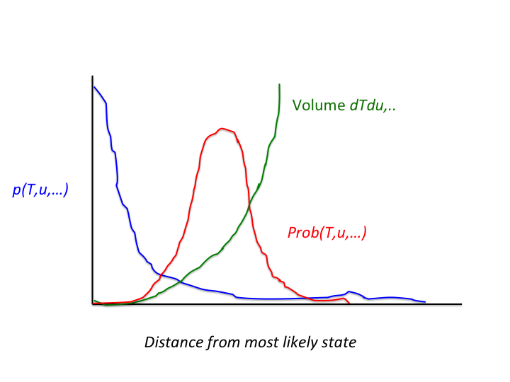
Figure 2. The blue curve shows the probability density of each weather event, with the most likely event having the largest value of the blue curve. Note that that curve decreases very rapidly with distance from this peak. The green curve denotes the volume of events that have the same distance from the most likely weather event. That curve grows very rapidly with distance from that most likely event. The red curve is the product of the two, and shows that the probability mass is not at the most likely weather event, but some distance away from that. For real weather models that distance can be huge …
So we find that the model runs should be very far away from the most likely weather event, in a rather narrow range it turns out. But what does that mean, and how do we get the models there? Very far away means that the total distance from the most likely weather event, measured in all variables and at all places that are in the model, is large. Looking at each variable individually, so for example the temperature in Reading, the distance is rather small. So, as shown in Figure 1, the differences are not that large if we only concentrate on a single variable. And how do we get the model runs there? Well, if the initial spread in the model runs was chosen to represent the uncertainty in our present estimate of the weather well, the model, if any good, should do the rest.
So you might ask what all this fuss is about. The answer is that to get the models starting in the right place to get the correct uncertainty is not easy. For that we need data assimilation, the science of combining models and observations. And for data assimilation these distances are crucial. But that will be another blog …