
By: Alan Grant

Science is an exciting career, although what you may consider to be exciting will depend on your field. Sometimes things get most exciting when what initially appears to be a frustrating problem turns into an interesting problem.
Our story starts with the decision to develop a new parametrization of the ocean surface boundary layer (OSBL). The main reason for this was to represent what is known as Langmuir turbulence (McWilliams et al, 1997), and as part of this, the depth of the base of the OSBL in the scheme would be determined using a prognostic equation. Simple models of the entraining boundary layer using a prognostic equation for the thickness of the boundary layer have been around for many years. However, a significant problem with the new scheme was to work out how to use a prognostic equation in a parametrization destined for use in a finite difference model. Eventually the new scheme was ready, and it was time to test it, initially using a one-dimensional model.
This scheme was developed as part of NERC’s Ocean Surface Mixing, Ocean Submesoscale Instabilities (OSMOSIS) project. As part of OSMOSIS, gliders were operated for a year in the area of the Porcupine Abyssal Plain (PAP, named after HMS Porcupine) observatory, off the continental shelf, to the south west of Ireland The scheme was assessed against this year of data.
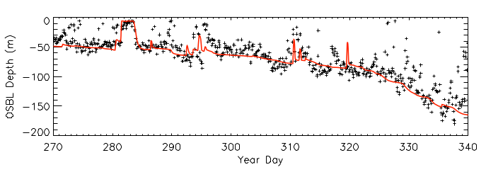
Figure 1 : Comparison between mixed layer depth determined from the gliders (symbols) and the boundary layer depth from the model (red curve) during the Autumn. The start date of the simulation is 23rd September.
The first test looked at the deepening of the boundary layer which occurs during the autumn. Figure 1 shows that there is good agreement between the boundary layer depth from the model and the mixed-layer depth obtained from the gliders. Over the seventy days of the simulation the thickness of the boundary layer increases from about 50m to 150m, due to entrainment.
 Figure 2 : Same as Figure 1 but for the winter. The start date of the simulation is 25th December
Encouraged by these results, we moved on to look at the performance of the model during the winter. Figure 2 shows the results of this comparison, and the reason for the frustration should be clear – during the winter the base of the boundary layer in the model gets much deeper than the mixed layer depth from the gliders. This deepening of the model boundary layer is due to entrainment, and there is little scope to simply tune the scheme to improve agreement, particularly given how well the scheme performs during the autumn.
This is where submesoscale motions enter in to our story. Submesoscale motions have scales between 100m to 10km, are generally associated with baroclinic instabilities, and are thought to restratify the upper ocean. While parametrizations of submesoscale motions are still crude, one developed by Fox-Kemper et al. (2008) is of particular interest. In this parametrization, the effect of the submesoscale motions is formulated in terms of a buoyancy flux. This makes it possible to directly couple the submesoscale parametrization to the equation for the thickness of the boundary layer in the new boundary layer scheme.
And so, our frustrating problem becomes an interesting problem, since we now need to think about how to couple parametrizations of two distinct processes. Preliminary tests of one way of doing this coupling are encouraging.
I forgot to mention, the new boundary layer parametrization has been implemented in the ocean model Nucleus for European Modelling of the Ocean (NEMO) where it gives overly deep boundary layers during the winter. The hope is that submesoscale motions will provide the solution to this problem.