
By: Ivo Pasmans
An anniversary is coming up in the family and I had decided to create a digital photo collage. In the process I was scanning a youth photo and noticed that the scan looked a lot less refined than the original. The resolution of my scanner, the number of pixels per square inch, is limited and since each pixel can record only one colour, details smaller than a pixel get lost in the digitization process. Now I doubt that the jubilees will really care that their collage isn’t of the highest quality possible, after all, it is the thought that counts. The story is probably different for a program manager of a million-dollar earth-observation satellite project.


Figure 1: (A) original satellite photo of sea ice. (B) Same photo but after 99.7% reduction in resolution (source: NOAA/NASA).
Just like my analogue youth photo, an image of sea-ice cover taken from space (Figure 1A) contains a lot of details. Clearly visible are cracks, also known as leads, dividing the ice into major ice floats. At higher zoom levels, smaller leads can be seen to emanate from the major leads, which in turn give rise to even smaller leads separating smaller floats, etc. This so-called fractal structure is partially lost on the current generation of sea-ice computer models. These models use a grid with grid cells and, like the pixels in my digitized youth photo, sea-ice quantities such as ice thickness, velocity or the water/ice-coverage ratio are assumed to be constant over the cells (Figure 1B). In particular, this means that if we want to use satellite observations to correct errors in the model output in a process called data assimilation (DA), we must average out all the subcell details in the observations that the model cannot resolve. Therefore, many features in the observations are lost.
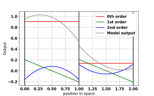
Figure 2: schematic example of how model output is constructed in DG models. In each of the two shown grid cells (separated by the black vertical lines), the model output is the sum of a 0th order polynomial (red), 1st order polynomial (green) and 2nd order polynomial (blue).
The aim of my research is to find a way to utilise these observations without losing details in the DA process for sea-ice models. Currently, a new sea-ice model is being developed as part the Scale-Aware Sea Ice Project (SASIP). In this model, sea-ice quantities in each grid cell are represented by a combination of polynomials (Figure 2) instead of as constant values. The higher the polynomial order, the more `wiggly` the polynomials become and the better small-scale details can be reproduced by the model. Moreover, the contribution of each polynomial to the model solution does not have to be the same across all of the model domain, a property that makes it possible to represent physical fields that vary very much over the domain. We are interested to make use of the new model’s ability to represent subcell details in the DA process and see if we can reduce the post-DA error in these new models by reducing the amount of averaging applied to the satellite observations.
As an initial test, we have set up a model without equations. There are no sea-ice dynamics in this model, but it has the advantage that we can create an artificial field mimicking, for example, ice velocity with details at the scales we want and the order of polynomials we desire. For the purpose of this experiment, we set aside one of the artificial fields as our DA target, create artificial observations from this one and see if DA can reconstruct the ‘target’ from these observations. The outcome of this experiment has confirmed our assumptions: when using higher-order polynomials, the DA becomes better in reconstructing the ‘target’ as we reduce the width over which we average the observations. And it is not just the DA estimate of the `target` that is improved, but also the estimate of the slope of the `target`. This is very promising: Forces in the ice scale with the slope of the velocity. We cannot directly observe these forces, but we can observe velocities. So, with the aid of higher-order polynomials we might be able to use the velocities to detect any errors in the in sea-ice forces.
High-resolution sea-ice observations definitely look better than their low-res counterparts, but to be able to use all details present in the observations DA has to be tweaked. Our preliminary results suggest that it is possible to incorporate scale dependency in the design of the DA scheme thus making it scale aware. We found that this allows us to take advantage of spatially dense observations and helps the DA scheme to deal with the wide range of scales present in the model errors.