Climate Action by Reducing Digital Waste

By: John Methven

Climate action has never been higher on the global agenda.

There is a pressing need to change our activities and habits, both at work and home, to steer towards a more sustainable future. National governments, public sector organizations and businesses are setting targets to achieve net zero carbon emissions by 2030. Immediately the term “carbon emissions” focuses attention on activities burning fossil fuel: driving a car, taking a train or catching a flight. However, when our Department first attempted its own carbon budget analysis in 2007, including the contribution of our activities to power consumption and carbon emissions far from Reading, we found that about 63% was attributable to computer usage compared with 24% business travel, 8% gas (heating) and 5% building electricity. Commuting to work was not included, although we are fortunate in that the majority of staff and students walk or cycle to work. The computing carbon cost was not even dominated by local power consumption by our computers (18%), or air-con in server rooms on site (7%), although the indirect carbon costs of the manufacture and ultimate waste disposal of those computers was not accounted for. The overwhelming contribution was from the extensive use of remote computing facilities (38%) – namely the supercomputers used to calculate weather forecasts, climate projections and to extend human knowledge in atmospheric and oceanic science.

What a conundrum! While improved weather forecasts save lives worldwide, through disaster risk mitigation, and also improve business efficiency, the daily creation of the forecasts is contributing to climate change which is increasing environmental risk. Back in 2008, many of the top 100 most powerful supercomputers were used for science, among them the leading global weather forecasting centres and international facilities enabling global climate modelling. Only 10 years on, the global cloud computing industry dwarfs the scientific supercomputing activity; even so, the global climate community takes supercomputing energy demands seriously. For example, scientists plan (Balaji et.al., Geos. Model Devel., 2017) to measure the energy consumed during the next generation simulations of future climate (CMIP6) that will contribute to the United Nations IPCC Sixth Assessment Report. As part of that effort they have developed new tools to share experiment design and simulations so that future computer usage can be minimized (Pascoe et.al., Geos. Model Devel. Disc., 2019). Many supercomputing facilities now have a renewable energy supply and there is even a Green500 list ranking supercomputers by energy efficiency.

 However, the revolutionary surge in digital storage has been outside the science sector: Gigabit magazine lists the top 10 cloud server centres in 2018 by capacity. The electricity consumption in the largest data centres worldwide is cited in the range 150-650 MW. Putting it into context, a single data centre can consume electricity equivalent to 2% of the entire UK electricity demand (34,000 MW)! Although some cloud server centres source electricity from renewables, such as dedicated hydro-electric plants, many do not and the total carbon footprint of cloud servers is huge. For example, Jones (Nature, 2018) states, “data centres use an estimated 200 terawatt hours (TWh) each year. That is more than the national energy consumption of some countries, including Iran, but half of the electricity used for transport worldwide, and just 1% of global electricity demand.” Some estimate that the carbon footprint from ICT (including computing, mobile phones and network infrastructure) already exceeds aviation. Although both sectors are expanding rapidly, cloud storage is expanding much faster with projections that over 20% of global electricity consumption will be attributable to computing by 2030. Much of the electricity is used to cool the computers, as well as power the hardware, and waste heat and water consumption are significant environmental issues. Although renewable power generation reduces the environmental impact, it is worth pausing for thought – what is all this data being stored?

Personal cloud storage is dominated by digital photos. Imagine you have been out with friends, your phone has uploaded the images as soon as it can sync to the cloud. No action required from you, but should you think twice? You have contributed to carbon emissions, and worse still the contribution will keep growing as long as you keep the data. How many of those photos will you look at again? Perhaps at least choose the best photos to keep and delete the rest?

In a work context, the storage for most businesses is dominated by email folders. Globally, 85% of email data volume is spam and 85% of that makes it into the inbox. Few people have time to go through their folders to delete unwanted messages and the volume mounts up. Emails are arriving continuously many with attachments, containing unsolicited images and hidden data on fonts (the content could have been relayed in plain text messages). Relentlessly piling up into a teetering heap of digital waste – requiring power to keep it alive – like a Doctor Who monster waiting just in case its master wants to visit tomorrow (artist’s impression?). Is the neglected monster sad? Perhaps a topic for AI fans.         

What can we do? What can you do? An effective contribution to climate action now would be to clear out your waste (somewhere out there on spinning disk), junk those emails and rubbish photos and feel good about it. Sorting tens of thousands of items into “keeps” and junk is a daunting task. Moving forward, wouldn’t it be good if all senders put a “use by date” on their emails and the recipient’s mail tool automatically deleted the message when expiry date was reached? Then we would know that the messages we send, even if unloved, at least do not contribute long-term to global digital waste.

All images have been spared in the creation of this article.


Posted in Climate, Climate change | Leave a comment

Teaching in China and some Good and Bad Teaching Practices

By: Hilary Weller

In April 2019 I visited the Nanjing University Institute of Information, Science and Technology (NUIST) where students are studying for a degree in Meteorology jointly between Reading and NUIST. Staff from Reading visit a couple of times a year to observe the lectures taught by the NUIST staff, teach the students and make new research links. Students study for years 1 and 2 in Nanjing and then come to Reading for their 3rd year. This is an interesting teaching challenge because Reading staff teach a random 2 weeks from 3 undergraduate modules.

I was sent PowerPoint files of seminar style slides — some bullet points, nice pictures and topics for discussion. I can imagine that these could make a terrific lecture if delivered by a charismatic visionary in the field who people would flock to hear talking, using the slides as illustrative prompts. But this is not me and these were not my slides. So, I needed to plan my teaching more carefully. I was asked to teach about measurements and instrumentation and tropical meteorology ­ a particular challenge as my area of expertise is numerical modelling of the atmosphere. I spent plenty of time learning about these subjects and planning my teaching.

I enjoyed learning about measurements of atmospheric radiation from Giles Harrison’s book Meteorological+Measurements+and+Instrumentation so much so that I have started making some YouTube teaching videos. and some online quizzes.

I observed loads of lectures while visiting NUIST, I have observed lectures in Reading, I have attended lectures as a student and I have delivered good and bad lectures myself. Based on this I will describe some difficult teaching situations and how they can be turned around, with or without preparation.

An Example: A Derivation

A lecturer (you?) plans to go through a derivation with students. In Meteorology it might be, for example, deriving thermal wind balance. You would like them to be able to provide a clear, thorough derivation, explaining each step-in full sentences. You have prepared some slides which outline the derivation but do not include complete sentences because you do not want to clutter your slides with words. You will say the linking sentences instead. This is a problem. You cannot expect the students to be able to write a good derivation if you haven’t given them a complete example. So, you might write it out in full for them and give them a copy of the lecture notes before class. But then they have nothing to do other than try to listen during your class. This breaks my first rule:

Make sure that the students have something to do during your class.

To give the students something to do, you go through the derivation on the board and ask them to volunteer what they think the next step might be. This is a natural way of explaining a derivation. However, if you do this with a class, one or two students may give you the answers you want, and the rest might be getting lost without asking questions. After the same person has answered a few questions, you direct your next question to a student who has so far remained quiet. Who cannot answer and is now humiliated. My next rule:

Do not single students out to answer questions.

These two rules seem to be mutually exclusive. I do not know the best way to teach while following these two rules, but I have some suggestions which will also work for large classes.

  1. Notes with gaps.

You could supply the students with printed notes with gaps and the students fill in the gaps during the lecture. They may copy the text for the gaps from the board or work it out for themselves. This way, the students take away a well written derivation, with all of the linking sentences between equations, and they have something to do and think about during the class. After you have gone through the derivation you could give them a couple of similar derivations to work through in pairs, asking for help if needed.

  1. Flipped classroom.

This teaching style can work very well but can also take a lot of preparation ­ you need to prepare material for the students to work through before and during class. The pre-class activity might be to read a section of a book or watch some SHORT videos. But you need to be careful not to overload the students. The activity before class should be straightforward and not take longer than the homework would have taken (which you must cancel). During class you can help them with more challenging material (assuming they have had time to go through the material before class). The tasks during class might be similar derivations or using the equation derived to explain some observed phenomena.

  1. Multiple choice questions.

I am keen on these as a quick way of engaging the whole class and they do not need to take a lot of preparation. When you come to a point when you would like to ask the class a question, you can instead write 3 or 4 possible answers on the board. They don’t all need to be plausible, you are just trying to encourage engagement. Then ask the students to show 1, 2, 3 or 4 fingers in front of their chest. That way you can see all the answers, the students cannot easily see each other’s answers (to avoid copying or humiliation) and every student is required to try to think of an answer. You may need to encourage them to guess and their answer doesn’t count for anything.

Another trap that people sometimes fall into:

If a student answers a question wrong, do not ask them to justify their answer. Ask someone else or explain it yourself.

  1. More challenging questions.

If you want to ask more challenging questions you will need to give the students more time to think about their answer, perhaps reread their notes or discuss with their neighbour. You should find out about “think-pair-share” or peer instruction. You can also use online quizzes which are popular with students but more time consuming to set up. Another rule:

Do not ask difficult or open-ended questions without giving the students time to think about, research or discuss an answer.

Also, make sure that your questions make sense and have well-defined answers. Check with a colleague to make sure that they are clear.

  1. Old fashioned teaching.

It may seem old fashioned but when I was teaching in China I asked the students to read a sentence in turn from the slides and fill in some simple gaps and copy text from the board. In the feedback, some of the students liked this approach, having an opportunity to practice speaking English and answer simple questions.

I would welcome more ideas for engaging all students while not humiliating anyone. Please leave a comment.

Posted in Academia, Climate, Teaching & Learning | Leave a comment

What sets the pattern of dynamic sea level change in the Southern Ocean?

By: Matthew Couldrey

Figure 1a: Multi-model mean projection of dynamic and steric (i.e. due to thermal and/or haline expansion/contraction) sea level rise averaged over 2081-2100 relative to 1986-2005 forced with a moderate emissions scenario (RCP4.5), including 0.18 m +/- 0.05 m of global mean steric sea level change. b: Root-mean square spread (deviation) of projections from the 21 model ensemble. (From Church et al 2013, their Figure 13.16)

Greenhouse gas forced climate change is expected to cause the global mean sea level to rise over the coming century, which will affect millions of people (Brown et al 2018) and cost trillions of US dollars (Jevrejeva et al. 2018). However, local factors are important in determining how much sea level change any particular place will experience, and these regional effects can double or entirely counteract the global mean change (Figure 1a). Furthermore, regional patterns of sea level change are challenging to predict, and climate models differ in their projections of this spatial pattern (Figure 1b). My research as part of the FAFMIP project (Flux Anomaly Forced Model Intercomparison Project, http://fafmip.org) aims to better understand why models disagree on the distribution of future sea level change.

Dynamic sea level (ζ) is the local sea surface height (above a geopotential surface) deviation from its global mean. Dynamic sea level is zero when averaged over the whole ocean surface, and its change over time (Δζ) shows the local change relative to the global mean. Therefore, positive values of Δζ indicate locations where sea level rise is larger than the global mean. Note that negative values of Δζ can correspond to locations of sea level rise (where the local change is smaller than the global mean, but still a rise) as well as sea level fall.

The hotspots in Figure 1b show locations where models from the previous generation of coupled climate (CMIP5) models disagree on the spatial pattern of sea level rise. The Southern Ocean is one of the regions where the pattern is uncertain, owing to a mixture of inter-model spread in 1) the ocean response to wind forcing, 2) changes in circulation, and 3) the redistribution of heat and freshwater. In an attempt to disentangle these causal processes, my research makes use of simulations where the oceans of several different models are forced with exactly the same changes in air-sea fluxes of heat, momentum (wind) and freshwater.

Figure 2: Thermal and haline contributions to dynamic sea level change across five Atmosphere-Ocean models, rows correspond to different models (named in left hand legends). Left panels: Zonally integrated change in ocean heat content per degree of latitude. Right panels: Zonal mean dynamic sea level change (Δζ, solid lines), and contributions from thermal expansion alone (dotted lines) and thermal plus haline effects (dashed lines).

The Southern Ocean dynamic sea level response is characterised by a strong north-south gradient, with relatively little change near the Antarctic continent and a northward-increasing rise (Figure 2, solid lines of right panels). This change arises partly because more heat gets added to lower latitudes of the Southern Ocean, peaking around 40 ˚S: note the ‘hump’ in the zonal ocean heat content change (left panels of Figure 2). However, the zonal dynamic sea level change (Δζ) shows a gradient then plateau (Figure 2, solid lines of right panels), rather than a ‘hump’, unlike the zonal heat content change. This is because of two reasons: the tendency of seawater to expand or contract changes markedly as you move from 70 ˚S to 45 ˚S. This means that the same heat input causes more dynamic sea level change at lower latitudes (where seawater is warmer) than at higher latitudes (where the temperature is lower). This ‘thermosteric’ or thermal expansion effect alone (Figure 2, dotted lines of right panels) would act to emphasise the ‘hump’ in sea level change suggested by the heat content change. In fact, the ‘haline contraction’ effect is what works against the thermal effects and flattens the hump into the gradient-plateau feature that we observe (Figure 2, dashed lines of right panels closely match the solid lines).

This work highlights that while ocean heat uptake sets the broad patterns of sea level change in the Southern Ocean, it’s the salinity changes that set the details. Furthermore, all the different models shown in Figure 2 were forced with the same pattern and magnitude of air-sea heat flux change. This means that the diversity in patterns of dynamic sea level change across different models largely arises due to differing ocean responses to climate change, rather than each model’s climate sensitivity (i.e. how much a particular model warms per unit of greenhouse gas emitted).

References

Brown, S., R. J. Nicholls, P. Goodwin, I. D. Haigh, D. Lincke, A. T. Vafeidis, & J. Hinkel, 2018, Quantifying Land and People Exposed to Sea-Level Rise with no Mitigation and 1.5∘C and 2.0∘C Rise in Global Temperatures to Year 2300, Earth’s Future, 6, 583-600, DOI 10.1002/2017EF000738

Church, J. A. , Clark, P. U., Cazenave, A., Gregory, J. M., Jevrejeva, S., Levermann, A., Merrifield, M. A., Milne,  G. A., Nerem, R. S., Nunn, P. D., Payne, A. J., Pfeffer, W. T., Stammer, D., and Unnikrishnan, A. S.: Sea Level Change, in: Climate Change 2013: The Physical Science Basis. Contribution of Working Group I to the Fifth Assessment Report of the Intergovernmental Panel on Climate Change, edited by: Stocker, T. F., Qin, D., Plattner, G.-K., Tignor, M., Allen, S. K., Boschung, J., Nauels, A., Xia, Y., Bex, V., and Midgley, P. M., Cambridge University Press, 2013. DOI 10.1017/CBO9781107415324.026

Jevrejeva, S., L. P. Jackson, A. Grinsted, D. Lincke, and B. Marzeion, 2018: Flood damage costs under the sea level rise with warming of 1.5 ∘C and 2 ∘C, Environ. Res. Lett., 13, DOI 10.1088/1748-9326/aacc76


Posted in Climate, Climate change, Climate modelling, Oceans | Tagged | Leave a comment

What do we do with weather forecasts?

By: Peter Clark

As I sat in the Kia Oval in Kennington having taken a day off to watch the first One Day International between England and Pakistan, I had plenty of time to appreciate the accuracy and utility of weather forecasts. The afternoon proved to be a microcosm of both the successes of modern weather forecasting and issues surrounding the use of forecasts in more serious applications (though I may well join in with the cries of “there’s nothing more serious than Cricket!”).

First question: to go to the match or not? When we bought the tickets 6 months ahead, we just had climatology to go on. Early May is a risk, but not very different from later in the season. By the time forecasts become available the question is then “is it worth turning up?” By the Friday five days before, there was a very strong consensus amongst computer forecasts that a cyclone would be tracking across England on the day, most likely during the first half of the day. In fact, the Met Office’s ‘deterministic’ forecast proved very accurate, with the continuous heavy rain passing through London by midday. However, behind the surface front close to the cyclone centre, cold air aloft was overrunning warmer air at the surface, which was given an additional boost as it came from the Atlantic and passed over land.  Warm (and moist) air beneath colder air leads to the likelihood of dreaded convective showers in the afternoon!

There have been real ‘revolutions’ in forecasting over the last few decades. At the centre lies the combination of vast improvements to computer power, more accurate computer models, vast increases in observations to ‘correct’ the data in the models, and development of much more powerful methods to use (or ‘assimilate’) those observations. An extratropical cyclone, or ‘low-pressure system’, is relatively large and long-lived. In this case, the system was at the small end of the scale and quite intense, roughly the size of England – say 500 km across with a life cycle of at least a day. 30 years ago, our computer models had to represent these systems with a grid of points not much better than 100 km apart (see the Met Office’s history of NWP, for example). Today our forecast models have little problem actually representing a cyclone. In practice, they are often predicted in forecast models even before there’s any clear sign of them in observations. While there will still be uncertainty in track and intensity, on the whole they are astonishingly well forecast several days ahead.

Here lies the problem. Showers are much smaller, say 10 km across with the core less than 1 km, and have a lifetime of an hour or so. These cannot even be directly represented in our global models. The most recent ‘revolution’ in forecasting has been the development of so-called ‘convection-permitting’ models (Clark et al. 2016). Regional models (with a grid spacing around 2 km) at last can represent showers, but not well. Something resembling showers can form and give us some very useful guidance on the probability that we’ll be affected by a shower. Such models are now helping produce more accurate flood forecasts, especially for smaller, faster reacting catchments (Dance et al. 2019). Within the ParaCon project we are working hard to find ways to improve the models.

Figure: Radar estimates of the surface rainfall rate at 17:00, 18:00 and 19:00 BST with inset showing the hail storm that hit the Kia Oval at 17:00 BST. (Courtesy of the Met Office). Showers are triggered along a ‘peninsular convergence’ line extending from Cornwall all the way to London that is present for several hours. Clearly, much depended on whether one was beneath or to one side of this.

The message was the same in the morning before the game. As the rain from the cyclone cleared, a high probability of seeing one or two showers or even thunderstorms during the afternoon – which is precisely what happened. We had a couple of flurries of not very intense rain, which did little to interrupt play, plus two hail storms; pea-sized hail fairly typical of a British summer shower. Each lasted about 5 minutes. The inset in the figure shows the hail storm that hit the oval around 17:00 BST. A mere speck on the scale of England, but locally extremely intense. A perfect forecast! However, a computer model run even a couple of hours before could not predict the precise shower hitting our precise location.

What more could we do? I spent the afternoon trying to look at the Met Office’s weather radar composites on my phone. A new rainfall picture is produced every 5 minutes. On the intermittent occasions when I could access data, the showers were very clearly tracked; interestingly they were forming along a broad ‘peninsular convergence’ line that could be tracked back to Land’s End. Along this line, air coming from either side of the south west peninsula meets and so is forced upwards, triggering showers (Golding et al, 2005). This is shown in the three radar images in the figure. Each is an hour apart, but this convergence line is very persistent. These lines were the topic of the COPE field campaign in 2013 (Leon, et al. 2016). This organisation by topography radically changed the overall predictability of the showers. The sharp-eyed reader might also notice an arc of showers moving east from central England into East Anglia, and it is probably no coincidence that the heaviest storm happened where this met the convergence line. Nevertheless, as we sat on the edge of this line, the best we could hope for several hours ahead was a realistic assessment of the probability of having a shower.

This example illustrates very well that the weather forecast is not the only piece in the jigsaw. First, and foremost, there is the investment in resilience; the Oval ground is very well prepared and drained, but there is a limit to what it can cope with. Similarly, investment in flood defences is often controversial, and the Environment Agency have recently announced that climate change is forcing a ‘new approach to flood and coastal resilience’ that may mean not investing in flood defences in some regions.

Second, there is preparedness. The available forecasts had prepared us well for the likelihood of showers. We equipped ourselves as well as we could. I kept a ‘weather eye’ on the radar, at least as far as technology allowed me. I could see the hail storms coming. In this case, the covers were deployed fast enough to protect the pitch and run-ups. Use of forecasts could enable the deployment of defences that take longer to deploy but ultimately save playing time. Currently, forecasts are used by the authorities to help emergency services prepare for likely (but rarely certain) flooding. How best to educate and prepare users including the public to respond to forecasts is one of the leading questions driving research, for example the World Meteorological Organisation’s ‘HIWeather Project’, which recognises the key importance of “better understanding by social scientists of the challenges to achieving effective use of forecasts and warnings” (HIWeather Impact plan). A key part of this is understanding the inevitability of false alarms. We have to be prepared to see play stopped because a forecast (in this case with a very short lead time) says there is a probability of a heavy shower. The price for not being pre-emptive may be the abandonment of the match. Which happened two and a half hours after the rain and hail stopped.

The modern challenge of forecasting is not just to improve the forecast (which may be an exercise in diminishing returns) but also to find ways to make sure that systems are in place to make full use of them and users are well-prepared to take action and understand the actions of others.

References:

Golding, B.W., Clark, P.A. and May, B., 2005, The Boscastle Flood: Meteorological Analysis of the Conditions Leading to Flooding on 16 August 2004, Weather60, 230-235,

Clark, P., Roberts, N., Lean, H., Ballard, S. P. and Charlton-Perez, C., 2016: Convection-permitting models: a step-change in rainfall forecasting. Meteorological Applications, 23 (2). 165-181. ISSN 1469-8080 doi: https://doi.org/10.1002/met.1538

Dance, S. L., Ballard, S. P., Bannister, R. N.Clark, P.Cloke, H. L., Darlington, T., Flack, D. L. A.Gray, S. L., Hawkness-Smith, L., Husnoo, N., Illingworth, A. J., Kelly, G. A., Lean, H. W., Li, D., Nichols, N. K.Nicol, J. C., Oxley, A., Plant, R. S., Roberts, N. M., Roulstone, I., Simonin, D., Thompson, R. J. and Waller, J. A., 2019: Improvements in forecasting intense rainfall: results from the FRANC (forecasting rainfall exploiting new data assimilation techniques and novel observations of convection) project. Atmosphere, 10 (3). 125. ISSN 2073-4433 doi: https://doi.org/10.3390/atmos10030125

Leon, D. C., French, J. R., Lasher-Trapp, S., Blyth, A. M., Abel, S. J., Ballard, S., Barrett, A., Bennett, L. J., Bower, K., Brooks, B., Brown, P., Charlton-Perez, C., Choularton, T., Clark, P., Collier, C., Crosier, J., Cui, Z., Dey, S., Dufton, D., Eagle, C., Flynn, M. J., Gallagher, M., Halliwell, C., Hanley, K., Hawkness-Smith, L., Huang, Y., Kelly, G., Kitchen, M., Korolev, A., Lean, H., Liu, Z., Marsham, J., Moser, D., Nicol, J., Norton, E. G., Plummer, D., Price, J., Ricketts, H., Roberts, N., Rosenberg, P. D., Simonin, D., Taylor, J. W., Warren, R., Williams, P. I. and Young, G., 2016: The COnvective Precipitation Experiment (COPE): investigating the origins of heavy precipitation in the southwestern UK. Bulletin of the American Meteorological Society, 97 (6). 1003-1020. ISSN 1520-0477 doi: https://doi.org/10.1175/BAMS-D-14-00157.1

Posted in Climate, Predictability, Weather forecasting | Tagged | Leave a comment

Rescuing the Weather

By: Ed Hawkins

Over the past 12 months, thousands of volunteer ‘citizen scientists’ have been helping climate scientists rescue millions of lost weather observations. Why?

Figure 1: Data from Leighton Park School in Reading from February 1903.

If we are to inform decisions about adapting to a changing climate we need to better understand the risk from extreme weather events, and whether this risk is changing. This requires long and detailed records of the weather. In the UK we are fortunate that meteorologists have recorded the weather across the country for over 150 years. However, most of their observations are still only available as the original paper copies, stored in large archives (Figure 1).

Currently, the only way to transform these observations into useful data is to manually transcribe them from paper to computer. This is an enormous task and would be much easier if it was performed by thousands of people, rather than just a single PhD student.

The WeatherRescue.org website has been set up to enable anyone to help. The first phase of the project recovered 1.5 million observations that were taken on the summit of Ben Nevis and in the nearby town of Fort William between 1883 and 1904. The volunteers then transcribed 1.8 million observations from more than 50 locations across Europe taken between 1900 and 1910. They are now digitising observations taken in the 1860s and 1870s.

So, what can we do with all this data?

Figure 2: Map of pressure observations in the ISPD database for 27th February 1903, including from ships (yellow), with newly rescued data (black) and locations where we have images of the observation logbooks, but the data has not yet been digitised (red).

As a case study, there was a very intense storm on February 26th-27th 1903 which hit Ireland and northern England, uprooting thousands of trees, causing significant structural damage and several fatalities. Hundreds of pressure observations taken across the UK during this storm are not in our digital climate databases. Figure 2 shows the existing data (yellow), newly rescued data (black) and potential data still waiting to be rescued (red) for the period of the intense storm.

Figure 3: The 26th-27th February 1903 storm in the 20th Century Reanalysis (left) and an estimate of how it would look with the new observations (right). The black contours are isobars, and the green shading shows confidence in their position.

The new data allows us to better reconstruct the path and intensity of the storm. Figure 3 shows how the storm appears in the new 20th Century Reanalysis (left) – it is too weak to cause the damage that we know occurred, and the image appears fuzzy because there is much uncertainty about the storm’s location. The right-hand panel shows how the storm should appear with the newly rescued observations (black dots in figure above) – more intense and more certain, with strong winds over eastern Ireland and northern England where the damage occurred. The minimum central pressure is now simulated to be around 955mb.

Severe windstorms are relatively rare but cause significant damage. We need to learn as much about them as possible which means delving back into the past. Thousands of volunteers are helping us determine how the weather changed hour-by-hour over a century ago and to learn about such extreme events. Anyone can help at WeatherRescue.org.


Posted in Climate, Data processing, Historical climatology, Outreach | Tagged , | Leave a comment

Mapping bio-UV products from space

By: Michael Taylor

Solar radiation arriving at the Earth’s surface in the UV part of the spectrum modulates photosynthetically-sensitive life on the land and in the oceans. UV radiation also drives important chemical reaction pathways in the atmosphere that impact air quality. It can cause DNA-damage in the epithelial cells of our skin and is a key factor for tuning the rate of Vitamin D production in our metabolism.

Solar UV radiation may be measured in radiometric units or spectrally-weighted to account for biologically-effective UV radiation doses. The Commission Internationale de l’Éclairage (CIE) defines the reference action spectrum for the ability of UV radiation as a function of wavelength to produce just perceptible erythema (colour change from the Greek word “ερυθρός” for red) in human skin. The standard erythemal dose (Jm-2) is equivalent to an erythemal radiant exposure of 100 Jm-2 (ISO 17166:1999). According to the Bunsen-Roscoe law of reciprocity (Bunsen & Roscoe, 1859), a given biological effect due to UV radiant exposure is directly proportional to the total energy dose given by the product of irradiance (Wm-2) and exposure time (s).

Figure 1: TEMIS erythemal UV dose products (kJ m-2) from KNMI/ESA (Van Geffen et al, 2017): daily “Clear sky” UV from SCIAMACHY/GOME-2, daily “cloud-modified” UV from SCIAMACHY/GOME-2 revealing the impact of a weather system over Sicily, and the global climatological “clear sky” June mean from GOME showing the impact of desert dust as revealed (lower right) by the global climatology of aerosol mixtures (Taylor et al, 2015).

Satellites like GOME, GOME-2 and SCIAMACHY have operational processing algorithms that retrieve erythemal UV dose (kJ m-2) once daily from top of the atmosphere irradiance measurements which are strongly affected by both cloud and atmospheric aerosol (Fig. 1).

Recent studies performed in the context of solar energy (Kosmopoulos et al., 2017; 2018), have revealed that atmospheric aerosol, and desert dust in particular, strongly attenuates solar radiation and the UV component arriving at the ground. In the context of increasing our global capacity for renewable energy with solar power as a major component, this is important. Since atmospheric aerosols reduce solar radiation by absorbing and scattering light and reduce the strength of the direct beam from which solar power generation is most efficient, they also cause forecast uncertainty. As a result, electricity supplied to national grids from solar power must balance the demand by coping with these unexpected fluctuations.

Figure 2: (a) Window functions used by KNMI/ESA to derive Bio-UV dose products from UV spectral irradiances and (b) the back-propagation neural network used to perform ground-based validation. See Zempila et al (2017) for details.

Nevertheless, it is straightforward to obtain biological ultraviolet (“Bio-UV”) products from the UV spectra retrieved at the ground. By applying weighting functions to the ultraviolet part of the irradiance spectra over the range 285-400 nm, important Bio-UV products like Vitamin D dose, DNA-damage dose and photosynthetically active radiation can be calculated. Satellite Bio-UV products from TEMIS (KNMI/ESA) have been successfully validated with high temporal resolution (1-minute) ground-based measurements by Zempila et al. (2017). Fig. 2 shows how the weighting functions vary with wavelength together with the neural network model developed to convert combinations of UV irradiances (I) and solar zenith angle (sza) to Bio-UV products for the ground-based validation.

Figure 3: Zoom sequence showing how the surface solar radiance spectra (280-2500 nm) retrieved under cloudy conditions from space with fast neural network radiative transfer solvers (Taylor et al., 2016) can be used to extract erythemal UV spectral irradiances for calculation of Bio-UV products as per Zempila et al., (2017).

While polar orbiting satellites like GOME, GOME-2, SCIAMACHY and OMI allow global maps of Bio-UV products to be generated, geostationary satellites like Meteosat Second Generation (MSG) provide high spatial resolution images of the Earth disc (3 km x 3 km) every few minutes and allow us to dramatically increase the frequency of the data. In support of this, an operational algorithm capable of retrieving the UV part of the solar spectrum at the surface was recently developed (Taylor et al., 2016). This was achieved with a synergistic model that uses both machine learning with neural networks and a look-up table of radiative transfer simulations to help unravel the complexity of the atmosphere. The model includes the effects of clouds, aerosols, ozone, elevation and surface albedo (Taylor et al; 2016; Kosmopoulos et al., 2017) and provides the surface global horizontal irradiance (GHI), direct normal irradiance (DNI) and diffuse horizontal irradiance (DHI) spectrum over the broad wavelength range 285-2700 nm. Application of the weighting functions of Fig. 2 to the UV part of the solar radiation spectrum can then provide global maps of Bio-UV products at high frequency. Fig. 3 illustrates how various UV products can be obtained from surface solar radiation spectra retrieved from space.

One of the most exci­ti­ng appl­icati­ons of being able to map UV spectral information ­from space is the potential for creating mob­ile appli­cat­ions that pull data from surface UV spectra data cloud computing resources and combi­ne them wi­th users’ GPS i­nformati­on to produce real-ti­me UV alerts to the general publi­c with unprecedented precision. By improving our capacity to map UV impact on the quality of life in the global ecosystem from space at high frequency, we will be better placed to monitor progress towards achievement of the UN’s sustainable development goals as we proceed to a more climate resilient society.

References

Bunsen, R., Roscoe, H. E., 1859: Photochemische untersuchungen. Annalen der Physik  184(10), 193-273, DOI: 10.1002/andp.18591841002

Kosmopoulos, P., S. Kazadzis, H. El-Askary, M. Taylor, A. Gkikas, E. Proestakis, C. Kontoes, M. M. El-Khayat, 2018: Earth-Observation-Based Estimation and Forecasting of Particulate Matter Impact on Solar Energy in Egypt. Remote Sens. 10(12), 1870, DOI: https://doi.org/10.3390/rs10121870

Kosmopoulos, P. G., S. Kazadzis, M. Taylor, E. Athanasopoulou, O. Speyer, P. I. Raptis, E. Marinou, E. Proestakis, S. Solomos, E. Gerasopoulos, V. Amiridis, 2017: Dust impact on surface solar irradiance assessed with model simulations, satellite observations and ground-based measurements. Atmos. Meas. Tech., 10(7), 2435-2453, DOI: 10.5194/amt-10-2435-2017

Taylor, M., P. G. Kosmopoulos, S. Kazadzis, I. Keramitsoglou, C. T. Kiranoudis, 2016: Neural network radiative transfer solvers for the generation of high resolution solar irradiance spectra parameterized by cloud and aerosol parameters. J. Quant. Spectrosc. Radiat. Transfer, 168, 176–192, DOI: 10.1016/j.jqsrt.2015.08.018

Taylor, M., S. Kazadzis, V. Amiridis, R. A. Kahn, 2015: Global aerosol mixtures and their multiyear and seasonal characteristics. Atmos. Environ., 116, 112–129, DOI: 10.1016/j.atmosenv.2015.06.029

Van Geffen, J., Van Weele, M., Allaart, M. and Van der A, R., 2017: TEMIS UV index and UV dose operational data products, version 2, KNMI Dataset, DOI:
10.21944/temis-uv-oper-v2

Zempila, M. M., J. H. van Geffen, M. Taylor, I. Fountoulakis, M. E. Koukouli, M. van Weele, R. J. van der A, A. Bais, C. Meleti, D. Balis, 2017: TEMIS UV product validation using NILU-UV ground-based measurements in Thessaloniki, Greece. Atmos. Chem. Phys., 17(11), 7157–7174, DOI: 10.5194/acp-17-7157-2017

Acknowledgements

I am very grateful to colleagues from the Tropospheric Emission Monitoring Internet Service (TEMIS) at KNMI and ESA for kindly making available plots of UV radiation monitoring products generated from the v2 processing algorithm, and to colleagues from the Greek national network for the measurement of ultraviolet solar radiation (uvnet.gr) for permission to present results from Zempila et al., (2017) using their ground-based NILU-UV multi-filter radiometer measurement data and associated UV dose data obtained from a Brewer MKIII spectrophotometer. I would also like to acknowledge colleagues from solea.gr with whom I collaborated with to develop the solar radiation neural network modeling aspects presented.

Posted in Climate, earth observation, Remote sensing, Solar radiation | Leave a comment

The sky is the limit – How tall buildings affect wind and air quality

By: Denise Hertwig

Based on current UN estimates, by 2050 over 6.6 billion people (68% of the total population) will be living in cities. Across the world, tall (> 50 m height) and super-tall (> 300 m) buildings already define the skylines of many large cities and will become increasingly more common outside of city centres to accommodate growing urban populations, especially when horizontal urban sprawl is geographically limited. For London, 2019 was declared the “year of the tall building” (NLA London Tall Buildings Survey 2019). At the moment, 541 buildings over 20 storeys (approx. 60 m in height) are planned or already under construction in the UK capital. Tall buildings are currently being built in 22 out of the 33 London boroughs and 76 of them are expected to be completed this year.

Tall buildings, in isolation or as clusters, affect the urban micro-climate of the local surroundings and the neighbouring region. The impact on aerodynamics (e.g. local flow distortions, long-range wake effects), radiation budget (e.g. shadowing, radiative trapping) and components of the surface energy balance (e.g. storage of heat in building materials, anthropogenic heat emissions) can be large compared to low-rise buildings. Such modifications challenge current modelling frameworks for urban areas. Urban land-surface models used in numerical weather prediction, for example, typically do not account for building-height variations. They also rely on the concept that the flow within the urban canopy is sufficiently decoupled from the flow aloft, which is not the case if tall buildings protrude deep into the urban boundary layer.

Figure 1: Normalised pollutant concentrations (a,b) in an idealised building array. Pollutants are released from point sources located (a) in the street canyon behind a tall building, (b) in an intersection upwind of the tall building. (c) Mean-flow streamlines near the tall building with colours showing the mean vertical velocity. The black arrow indicates the upwind flow direction. Data are results from large-eddy simulations by Fuka et al. (2018) for the DIPLOS project.

Similarly, operational urban air quality and dispersion models do not usually account for tall-building effects (Hertwig et al. 2018). Tall buildings strongly change pedestrian-level winds in the surrounding streets and the flow field above the roofs of the low-lying buildings. This affects pollutant pathways and the overall ventilation potential of cities. Pollutants released near the ground in a street canyon on the leeward side of a tall building (Fig. 1a) can be rapidly lifted out of the building canopy by updrafts (Fig. 1c). Although the pollutants are emitted at the ground, the tall building causes a large proportion of the released mass to be transported above the roofs of the low-rise neighbourhoods, thereby reducing street-level pollution. A pollutant source located in an upwind intersection leads to drastically different results (Fig. 1b). The downdrafts on the windward side of the tall building result in strong horizontal flow out of the upwind street canyon (Fig. 1c). This outflow shifts the pollutants away from their release point in the intersection, creating a virtual source location in the adjacent street canyon and deteriorating air quality in the streets downwind.

Figure 2: (a) Building heights and (b) wind-tunnel model buildings of the neighbourhood between Waterloo station and Elephant & Castle in London (MAGIC project study area). Wind-tunnel measurements of the wake behind the central tall building (81 m height) in isolation and together with the low-rise building canopy shown in terms of (c) height profiles of flow speeds at several sites downwind of the tall building, (d) velocity differences to the ambient (undisturbed) flow with downwind distance at several heights. Details in Hertwig et al. (2019).

Flow interactions between tall and low-rise buildings also change the structure of the momentum deficit region (wake) that forms behind tall buildings. Wake models used for local air-quality predictions currently do not account for such interactions as they were derived for isolated buildings. Wind-tunnel experiments in a realistic scale model of the area between the Waterloo and Elephant & Castle stations in London (Fig. 2a,b) documented the strong impact of the canopy on tall-building wakes (Hertwig et al. 2019). Compared to tall buildings in isolation, the presence of a low-rise canopy displaces the wake vertically (Fig. 2c), so that flow speeds are reduced over longer distances downwind well-above the canopy (Fig. 2d). In the case shown, the wake extends over distances larger than 5 times the height of the tall building (i.e. > 400 m). The increasing spatial resolution (of the order of 100 m) of mesoscale and microscale atmospheric models means that tall-building wakes no longer are subgrid-scale phenomena, but have an impact at the grid-scale. Understanding and quantifying tall-building impacts on the boundary layer over cities is essential to identify needs for model refinements.

References

Fuka, V., Z.-T. Xie, I.P. Castro, P. Hayden, M. Carpentieri, A.G. Robins, 2018: Scalar fluxes near a tall building in an aligned array of rectangular buildings. Boundary-Layer Meteorology 167, 53–76, DOI: 10.1007/s10546-017-0308-4

Hertwig, D., L. Soulhac, V. Fuka, T. Auerswald, M. Carpentieri, P. Hayden, A. Robins, Z.-T. Xie and O. Coceal, 2018: Evaluation of fast atmospheric dispersion models in a regular street network. Environmental Fluid Mechanics 18, 1007–1044, DOI: 10.1007/s10652-018-9587-7

Hertwig, D., H.L. Gough, S. Grimmond, J.F. Barlow, C.W. Kent, W.E. Lin, A.G. Robins and P. Hayden, 2019: Wake characteristics of tall buildings in a realistic urban canopy. Boundary-Layer Meteorology, DOI: 10.1007/s10546-019-00450-7 (in press)

Posted in Boundary layer, Climate, Urban meteorology | Leave a comment

Balloon measurements at Stromboli suggest radioactivity contributes charge in volcanic plumes

By: Martin Airey

Volcanic lightning is an awe-inspiring and humbling display of nature’s power. It results from the breakdown of large electric fields that are generated within the volcanic plume. The processes that result in the accumulation of charge are varied and complex and by no means fully understood. Current knowledge of the key established mechanisms that are known to contribute to plume charging centre around the role played by ash. These mechanisms fall broadly into the categories of fractoemission and triboelectrification (Mather and Harrison, 2006). Fractoemission is the release of neutral and charged (electrons, positive ions, and photons) particles from fracture surfaces as magma fragments upon eruption (James et al., 2000); these particles may then interact with ash and aerosols to impart a net charge. Triboelectrification is a mechanism by which charge is transferred between the ash particles as they collide.

When charge has been produced, it must then be separated in order for an electric field to develop and a discharge to occur. The plume is a dynamic and chaotic environment, where primitive constituents of the magma, such as solid particles, gases, and metal species are mixed with atmospheric material as it is entrained by the plume. Above the initial jet region, thermal buoyancy-driven dynamics enable the plume to grow to an altitude at which neutral buoyancy is attained. Within this setting, charged aerosols and charged ash grains settle differently resulting in the separation of positively and negatively charged regions in the plume (Mather and Harrison, 2006), which can ultimately cause a discharge to occur.

But what if there are other additional mechanisms that contribute to either the charging or separation processes? As it is a complex, rapidly evolving, multiphase environment, there is the potential for many other chemical and physical interactions occurring within the plume that may currently be overlooked by this simplistic view. To test this, sensors and instrumentation developed at Reading over many years for deployment on weather balloons was combined through a NERC-funded project into a disposable modular payload called VOLCLAB (VOLCano LABoratory). The range of sensors that can be incorporated into the VOLCLAB package includes an optical backscatter droplet detector, a charge sensor, a sulphur dioxide sensor, an oscillating microbalance particle collector, and a turbulence sensor.


View from Stromboli’s summit into the vent complex showing the gas-rich plumes

In September 2017, a team of scientists from the University of Reading, Ludwig Maximillians Universität (Munich), and the University of Bath set off to Stromboli on fieldwork funded by National Geographic, equipped with VOLCLAB sensors, radiosondes, balloons, a thunderstorm detector, and lots of helium. Stromboli was an ideal choice for this expedition as it erupts frequently (several times an hour) and produces a wide range of plume types ranging from ash-rich to predominately gaseous. By launching these instruments directly into the plumes, in situ measurements may be acquired from all these plume types. The two-week long campaign required a daily hike to the summit at 900 m, often with very heavy kit. Many sensor-equipped balloons were launched from the summit with a range of success in encountering a plume, and VOLCLAB packages were deployed in fixed locations around the summit to continually record passing plumes.

   Martin Airey (holding VOLCLAB package) and Corrado Cimarelli

                 Keri Nicoll, Kuang Koh, and Martin Airey

Most interesting was the discovery of significant electric charge in plumes that contained negligible or no ash. This led to the investigation of what might be causing this unexpected charging mechanism. It is widely known that volcanoes emit a broad range of chemical products (Allard et al, 2000), one of which is radon, which is produced in high concentrations from all volcanoes. Radon is routinely monitored at many volcanoes, including Stromboli, which is known to constantly emit very large quantities through the soil near the vents, and even more during eruptions (Cigolini et al, 2009). As radon radioactively decays, it increases the charge present by ionising the air. This additional source of charge, inferred for the first time with these new direct measurements inside gaseous plumes, will inevitably contribute to the overall charge structure and may affect the likelihood of lightning strikes.

The original open access article, published in Geophysical Research Letters, may be found at: https://agupubs.onlinelibrary.wiley.com/doi/full/10.1029/2019GL082211

And additional press can be found in the following links:
Science: https://www.sciencemag.org/news/2019/03/volcanic-lightning-may-be-partially-fed-earth-s-natural-radioactivity
New York Times: https://www.nytimes.com/2019/03/29/science/volcanoes-lightning-radon-gas.html
Atlas Obscura: https://www.atlasobscura.com/articles/mount-stromboli-volcano-science
The VOLCLAB package covered in Meteorological Technology magazine: 
http://viewer.zmags.com/publication/235ac328#/235ac328/56
Some footage of the fieldwork was also included in the Arte documentary “Living with Volcanoes” from around 7 minutes: 
French: https://www.arte.tv/fr/videos/069786-010-A/des-volcans-et-des-hommes-iles-eoliennes/
German: https://www.arte.tv/de/videos/069786-010-A/leben-mit-vulkanen/

References:

Allard, P., Aiuppa, A., Loyer, H., Carrot, F., Gaudry, A., Pinte, G., et al. (2000). Acid gas and metal emission rates during long‐lived basalt degassing at Stromboli volcano. Geophysical Research Letters, 27(8), 1207–1210. https://doi.org/10.1029/1999GL008413

Cigolini, C., Poggi, P., Ripepe, M., Laiolo, M., Ciamberlini, C., Delle Donne, D., et al. (2009). Radon surveys and real‐time monitoring at Stromboli volcano: Influence of soil temperature, atmospheric pressure and tidal forces on 222Rn degassing. Journal of Volcanology and Geothermal Research, 184(3–4), 381–388. https://doi.org/10.1016/j.jvolgeores.2009.04.019

James, M. R., Lane, S. J., & Gilbert, J. S. (2000). Volcanic plume electrification—Experimental investigation of fracture charging mechanism. Journal of Geophysical Research, 105(B7), 16,641–16,649. https://doi.org/10.1029/2000JB900068

Mather, T. A., & Harrison, R. G. (2006). Electrification of volcanic plumes. Surveys in Geophysics, 27(4), 387–432. https://doi.org/10.1007/s10712‐006‐9007‐2


Posted in Climate, Convection, Measurements and instrumentation | Tagged | Leave a comment

Convective self-aggregation: growing storms in a virtual laboratory

By: Chris Holloway

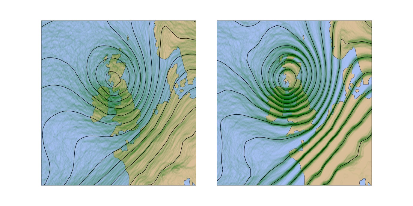
Figure 1: An example of convective self-aggregation from an RCE simulation using the Met Office Unified Model at 4km grid length with 300 K SST.  Time mean precipitation in mm/day for (a) Day 2 (still scattered), and (b) Day 40 (aggregated).  Note that the lateral boundaries are bi-periodic, so the cluster in (b) is a single organised region.  Adapted from Holloway and Woolnough (2016).

Convective self-aggregation is the clumping together of isolated convective cells (rainstorms) into organised regions in idealised computer simulations.  This storm clustering may not seem all that unusual, but it is surprising because self-aggregation occurs in simulations of “radiative-convective equilibrium” (RCE) in which boundary conditions are homogeneous (sea surface temperature [SST] is constant in space and time), there is no imposed mean wind, and planetary rotation is set to zero (e.g., Figure 1).  In other words, there is no external cause of the clustering of convection in self-aggregation (hence the “self” prefix).  Instead, internal feedbacks such as cloud-radiation interactions and surface-flux feedbacks are key (Wing et al.2017 and references therein).

Figure 2: Satellite estimates of average fractional cover vs total Cold Cloud Area for a given domain-mean precipitation rate (R) range and for ranges of the “SCAI” aggregation index between 0.00 and 0.35 (red, aggregated), between 0.35 and 0.70 (black, intermediate), and between 0.70 and 1.50 (blue, disaggregated); t stands for optical thickness. Shaded regions indicate the 90% confidence interval. (a)–(c) thick anvil, (d)–(f) optically thin anvil.  Adapted from Stein et al. (2017).

While self-aggregation is intellectually interesting, many scientists are sceptical of the relevance of this phenomenon for real weather and climate.  After all, the real world has plenty of inhomogeneity in surface temperature as well as rotation and vertical wind shear.  However, organised tropical convection in real-world observations shows many similarities to self-aggregated convection in idealised simulations: for more aggregated conditions the mean state has lower relative humidity, outgoing longwave radiation (OLR) is larger, and anvil cloud amount is reduced (Holloway et al. 2017 and references therein).  For instance, work at the University of Reading using satellite observations has shown that optically thin anvil cloud cover decreases as convection becomes more aggregated, which could have implications for climate (Figure 2).    More realistic convective-scale simulations of organised tropical convection (with observed SSTs, rotational effects, and wind shear effects) also provide evidence that cloud-radiation feedbacks act to maintain organisation and reduce the mean relative humidity (Holloway 2017).   Other real-world forms of organised tropical convection, including the Madden-Julian Oscillation (MJO), tropical cyclones, and the Intertropical Convergence Zone (ITCZ) all show cloud-radiative feedbacks and moisture-convection feedbacks that resemble processes important for convective self-aggregation in idealised computer simulations.

The potential impact of convective aggregation on climate is an area of active research and debate.  Some idealised computer experiments show stronger self-aggregation with warmer SSTs sea surfaces, but others do not (Wing 2019).  If aggregation were to increase with increasing SST, this would likely be a slightly negative feedback for global warming, meaning it would allow for slightly less warming for a given increase in carbon dioxide concentrations, but this is also an active area of research and debate.  Aggregation tends to be weaker and more variable in simulations that include coupled ocean models (e.g. Hohenegger and Stevens 2016, Coppin and Bony 2017), so this is another area that needs more extensive research. 

Studying convective aggregation enables the scientific community to generate and test hypotheses and isolate mechanisms about fundamental processes that are potentially important for convective organisation, but which can be difficult to disentangle in more realistic settings.  Even if studies eventually demonstrate how self-aggregation is not an adequate framework for some climate problems, this will also be a form of important progress.  The Radiative-Convective Equilibrium Model Intercomparison Project (RCEMIP) is bringing scientific institutions together to compare self-aggregation at different model resolutions, domains and SSTs in order to facilitate further research into this exciting topic.  At Reading, Met Office Unified Model convection-permitting simulations have been performed and submitted to RCEMIP in association with the joint NERC-Met Office ParaCon project which seeks to greatly improve the representation of convection in weather and climate models.   RCEMIP and other research efforts will increasingly apply new concepts emerging from idealised simulations to the complex interactions between convection, moisture, clouds, radiation, surface fluxes, circulations and climate.

References:

Coppin, D., and S. Bony, 2017: Internal variability in a coupled general circulation model in radiative‐convective equilibrium, Geophysical Research Letters, 44, 10, 5142-5149, https://doi.org/10.1002/2017GL073658.

Hohenegger, C., and Stevens, B., 2016: Coupled radiative convective equilibrium simulations with explicit and parameterized convection. J. Adv. Model. Earth Syst., 8, 1468–1482, doi:10.1002/2016MS000666.

Holloway, C. E., 2017: Convective aggregation in realistic convective- scale simulations, J. Adv. Model. Earth Syst., 9, 1450–1472, doi:10.1002/ 2017MS000980.

Holloway, C. E., A. A. Wing, S. Bony, C. Muller, H. Masunaga, T. S. L’Ecuyer, D. D. Turner, and P. Zuidema, 2017: Observing convective aggregation.  Surveys in Geophysics, 38: 1199. doi:10.1007/s10712-017-9419-1. 

Holloway, C. E., and S. J. Woolnough, 2016: The sensitivity of convective aggregation to diabatic processes in idealized radiative-convective equilibrium simulations.  J. Adv. Model. Earth Syst., 8, 166–195, doi:10.1002/2015MS000511.

Stein, T. H. M., C. E. Holloway, I. Tobin, and S. Bony, 2017: Observed relationships between cloud vertical structure and convective aggregation over tropical ocean.  J. Climate, 30, 2187–2207. 

Wing, A. A., 2019: Self-Aggregation of Deep Convection and its Implications for Climate. Curr. Clim. Change Rep., 5: 1. https://doi.org/10.1007/s40641-019-00120-3.

Wing, A. A., K. Emanuel, C. E. Holloway, and C. Muller, 2017: Convective self-aggregation in numerical simulations: A review.  Surveys in Geophysics, 38: 1173. https://doi.org/10.1007/s10712-017-9408-4.


Posted in Climate, Climate modelling, Numerical modelling, Tropical convection | Leave a comment

Modelling Ice Sheets in the global Earth System

By: Robin Smith

As Till wrote recently, our national flagship climate model (UKESM1, the UK Earth System Model) has been officially released for the community to use, after more than six years in development by a team drawn from across the NERC research centres and the Met Office. The most unique capability of the UKESM effort isn’t included in that release however: UKESM1 can also be made to interactively simulate the evolution of the massive ice sheets of Greenland and Antarctica.

On millennial timescales, the growth and decay of ice sheets play one of the most fundamental roles in determining the climate of the Earth – think of the ice-age cycles of the last million years. But ice sheets aren’t just for the paleoclimate people. Loss of mass from ice sheets accounts for around a third of the currently observed global mean sea level rise and their contribution is expected to increase and dominate the sea level budget in the coming decades and centuries (Church et al. 2013). The climate change impact from ice sheets isn’t limited to sea level rise either, with ice melt input to the ocean linked to a range of wide climate change problems (Golledge et al. 2019).

Back near the start of this project I wrote in this blog about plans for the ice sheets in UKESM and some of the challenges that we were facing. Since then we’ve implemented a system of online climate downscaling over ice sheets in the Met Office Unified Model, taught the NEMO (Nucleus for European Modelling of the Ocean) ocean model to move its boundaries (a little) as it runs without becoming unstable and built a whole framework of Python code to transfer fields between the BISICLES (Berkley Ice Sheet Initiative for Climate Extremes) ice sheet model and the rest of the climate system. The whole system adds additional layers of complexity to what is already one of the most sophisticated climate models in the world. It’s all still a bit rough around the edges, which is why this isn’t included in the main UKESM1 release, but there is finally a functioning coupled climate-ice model that can do things that no other state of the art climate model can do.

 Figure 1: Surface Mass Balance (SMB) (the balance between accumulating and melting snow) estimated for Greenland in UKESM (blue and black lines) compared with the output from a specialised regional climate model (red line, Noel et al. 2018). UKESM captures the observed downturn in SMB at the end of the 1990s, often linked with decadal variability in the North Atlantic. The coupled ice sheet component additionally models the dynamic flow and calving rate of the ice sheet to give a complete estimate of how the ice mass will evolve.

So, has it all been worth it? What are we going to do with this model now we’ve made it? Whilst there are many open questions around the stability of the large ice sheets and how they interact with the climate around them, our first goal will be completion of a set of coupled climate—ice simulations for the Ice Sheet Model Intercomparison ISMIP6, an international model intercomparison that will provide projections of 21st century ice sheet mass loss. Early results from UKESM with our new online downscaling for the ice compare very well to regional climate model results (Figure 1) and suggest that additional surface melt of Greenland alone could be adding another millimetre to global-mean sea level every year by 2050.

Figure 2: Pine Island Glacier on Antarctica is observed to be thinning and retreating rapidly, most likely in response to ocean warming underneath its ice shelf. With the interactive ice in  UKESM we can model how the ocean melts the shelf away (top right), the flow of the glacier supplying new ice to the region (top left) and predict the overall rate of retreat. These are early results but show promise.

The most exciting new science we want to tackle with the ice in UKESM1 sits at the other end of the globe, however. There are many theories about how the floating ice shelves that fringe Antarctica respond to changes in ocean conditions, and how the flow of the grounded ice upstream will respond, but the uncertainties are enormous. Estimates of the resulting contribution to global mean sea level rise at 2100 range from centimetres to metres (see Edwards et al. 2019 for a recent perspective). This is an inherently coupled problem whose physics simply cannot be understood by modelling any one part of the system in isolation. Like all complex problems, it’s also going to be very hard – there are poorly-observed, crucial details in each component that can significantly alter the final outcomes – and we’re not pretending that one model is going to lead us straight to the answers. For one thing, there are long-standing biases in the climate simulation of the Met Office models in the high southern latitudes that will need to be improved before we are really simulating the processes against the right background.  But with UKESM1 we’re now getting our hands on some tools that can start to see the coupled atmosphere-ocean-ice physics evolving together for the first time (Figure 2), and that’s a very promising development.

References:

Church, J.A., and Coauthors, 2013: Sea Level Change. Climate Change 2013: The Physical Science Basis. Contribution of Working Group I to the Fifth Assessment Report of the Intergovernmental Panel on Climate Change, Stocker, T.F., D. Qin, G.-K. Plattner, M. Tignor, S.K. Allen, J. Boschung,  A. Nauels, Y. Xia, V. Bex and P.M. Midgley, Eds. Cambridge University Press, 1137-1216

Edwards, T.L., M.A. Brandon, G. Durand, N.R. Edwards, N.R. Golledge, P.B. Holden, I.J. Nias, A.J. Payne, C. Ritz & A. Wernecke, 2019: Revisiting Antarctic ice loss due to marine ice-cliff instability. Nature, 566, 58-64, https://doi.org/10.1038/s41586-019-0901-4

Golledge, N.R., E.D. Keller, N. Gomez, K.A. Naughten, J. Bernales, L.D. Trusel & T.L. Edwards, 2019: Global environmental consequences of twenty-first-century ice-sheet melt. Nature, 566, 65-72, https://doi.org/10.1038/s41586-019-0889-9

Noël, B. and Coauthors, 2018: Modelling the climate and surface mass balance of polar ice sheets using RACMO2 – Part 1: Greenland (1958–2016). The Cryosphere, 12, 811-831, https://doi.org/10.5194/tc-12-811-2018

Posted in Arctic, Climate, Climate modelling, Cryosphere, Numerical modelling | Tagged | Leave a comment