Multi-fluids Modelling of Convection

By: Hilary Weller

Atmospheric convection – the dynamics behind clouds and precipitation – is one of the biggest challenges of weather and climate modelling. Convection is the driver of atmospheric circulation, but most clouds are smaller than the grid size and so cannot be represented accurately or at all. Consequently, all but the highest resolution models use convection parameterisations – statistical representations which estimate the heat and moisture that would be produced and transported by clouds if they were resolved. These parameterisations have become sophisticated, estimating the mass that is transported upwards and how this will influence the momentum, temperature, moisture and precipitation. Without these parameterisations climate models dramatically fail. However, there are still big problems with these parameterisations; they tend to produce unrealistic hot columns of air and the main regions of convection in the tropics are usually misplaced (see Figure 1). These are large heat sources for the global atmosphere and so errors in these locations have knock-on effects across the globe.

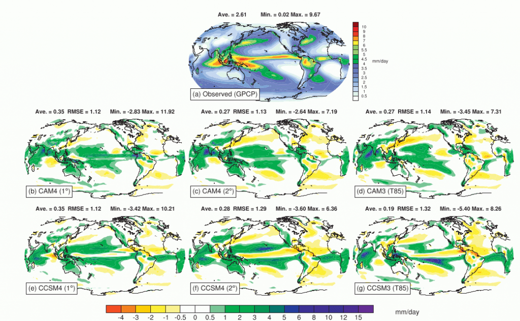
Figure 1: Fig 11 from Neale et al, (2013) showing “Annually averaged (a) observed precipitation from GPCP (1979–2003) and model precipitation biases (mm day 21 ) in AMIP-type experiments for (b) CAM4 at 18, (c) CAM4 at 28, and (d) CAM3 at T85, and in fully coupled experiments for (e) CCSM4 at 18, (f) CCSM4 at 28, and (g) CCSM3 at T85.”

There are two assumptions made in convection parameterisations that could be to blame for their poor performance. Firstly, there is no memory of the properties of convection from one time-step to the next. The convection properties are calculated each time step from scratch as if there had been no convection in the previous time step. Secondly, although there is a class of convection scheme called “mass flux”, convection schemes do not actually transport air upwards. They transport the heat, moisture and momentum but the distribution of mass in the vertical is not changed by the convection scheme. Removing these assumptions is quite tricky. You realise that what you need to do is solve the same equations of motion in clouds and outside clouds, but these need to be modelled separately because the clouds are such a small fraction of the total volume. This is the multi-fluid approach. Separate equations for velocity, temperature, moisture, and volume fraction are solved for the air in clouds and the environmental air, outside clouds. As the clouds and the environment are interwoven, we assume that they share the same pressure.

John Thuburn and I are working on making this approach work as part of the NERC/Met Office Paracon project to develop big changes to the way that convection is parameterised in order to remove some of the less realistic assumptions (Thuburn et al, 2018, Weller and McIntyre, 2019). As ever, it is proving more difficult than we expected. We knew that we would need to solve simultaneous equations for the properties in and outside the clouds and that these would need to be simultaneous with the single pressure. I naively thought that this would be sufficient and that my expertise in this area would make it possible whereas convection modellers are usually less familiar with this simultaneous solution procedure. However, it turns out that the multi-fluid equations can be unstable. They are easy to stabilise but the stabilisation can have the effect of making the two fluids behave as one which defeats the purpose. We need to make the two fluids move through each other. John has made some good progress on this (Thuburn et al, 2019).

The multi-fluid equations need transfer terms to transfer air in and out of the clouds. These are not a mystery. Traditional parameterisations predict these transfers, and these have been thoroughly validated and tested. However, the multi-fluid equations are sensitive to these transfer terms and do not behave in the same way as the traditional parameterisations. We also want to base the transfers on the sub-grid scale variability both inside and outside the cloud so that a cloud is formed if some of the air in a grid box is ready to rise and condense out water. There is plenty to do.

While the multi-fluids team from the Paracon project have been working on simultaneous solutions of equations for in and outside clouds, ECMWF thought that they would try a more direct approach – simply adding a term to the continuity equation based on the mass flux predicted by their traditional parameterisation (Malardel and Bechtold, 2019). This was also the approach taken by Kuell and Bott (2008). The problem with this approach is that it will be unstable if a large fraction of a grid box is cloudy. However, ECMWF and Kuell and Bott (2008) have not reported any stability problems, although the ECMWF approach did ensure that only a small fraction of each grid box is transported by the convection scheme. The results so far seem promising. However, to be able to increase the resolution and run with sufficiently long time steps so that the model is competitive, we will need the multi-fluid approach.

References:

Kuell, V., and A. Bott, 2008: A hybrid convection scheme for use in non-hydrostatic numerical weather prediction models. Meteorol. Z. 17 (6), 775-783, https://doi.org/10.1127/0941-2948/2008/0342

Malardel, S. and Bechtold, P. (2019), The coupling of deep convection with the resolved flow via the divergence of mass flux in the IFS. Q J R Meteorol Soc. https://doi:10.1002/qj.3528

Neale R.B., J. Richter, S. Park, P.H. Lauritzen, S.J. Vavrus, P.J. Rasch, M. Zhang, 2013: The Mean Climate of the Community Atmosphere Model (CAM4) in Forced SST and Fully Coupled Experiments. J. Climate., 26, 5150-5168, https://doi.org/10.1175/JCLI-D-12-00236.1

Thuburn, J., G.A. Efstathiou, R.J. Beare, 2019: A two‐fluid single‐column model of the dry, shear‐free, convective boundary layer. Quart. J. Roy. Meteor. Soc., https://doi.org/10.1002/qj.3510

Thuburn, J., H. Weller, G.K. Vallis, R.J. Beare, and M. Whitall, 2018: A framework for convection and boundary layer parameterization derived from conditional filtering.  J. Atmos. Sci., 75 (3), 965-981, https://doi.org/10.1175/JAS-D-17-0130.1

Weller, H., W. McIntyre, 2019: Numerical Solution of the Conditionally Averaged Equations for Representing Net Mass Flux due to Convection. Quart. J. Roy. Meteor. Soc., https://doi.org/10.1002/qj.3490

Posted in Climate, Convection, Numerical modelling | Leave a comment

SuPy: An urban land surface model for Pythonista

By: Ting Sun

Python is now extensively employed by the atmospheric sciences community for data analyses and numerical modelling thanks to its simplicity and the large scientific Python ecosystem (e.g., PyData community). Although I cherish Mathematica as my native programming language (like Mandarin as my mother tongue), I can see I have coded much more in Python than in Mathematica over the past year for my urban climate research.

One of the core tasks in urban climate research is to build climate resilience, where climate information at various spatiotemporal scales is an essential prerequisite. To obtain such climate information, accurate and agile modelling capacity of the urban climate is essential. Urban land surface models (ULSM) are widely used to simulate urban-atmospheric interactions by quantifying the energy, water and mass fluxes between the surface and urban atmosphere.

One widely used and tested ULSM, the Surface Urban Energy and Water balance Scheme (SUEWS) developed by Micromet@UoR, requires basic meteorological data and surface information to characterise essential urban features (i.e., urban surface heterogeneity and anthropogenic dynamics). SUEWS enables long-term urban climate simulations without specialised computing facilities (Järvi et al., 2011; 2014a; Ward et al., 2016). SUEWS is regularly enhanced and tested in cities under a range of climates worldwide.

Figure 1: SUEWS-Centred workflow for urban climate simulations

The typical workflow of conducting a SUEWS simulation may consist of a few steps (Figure 1), where several pre- and post-processing procedures can in fact be easily done by Python. However, one inevitable step that often bothers me is that the change of a single parameter may lead to another loop of the above workflow, which is somewhat annoying and tedious as you need to switch back and forth between numerous applications again and again.

Given the glue-like ability of Python, I started the project SuPy (SUEWS in Python) to use Python as a central tool to build a SUEWS-back-ended urban land surface model since the development of SUEWS v2017b. After several months of development and testing, I’m very pleased to release SuPy (Sun 2019; Sun and Grimmond 2019) via PyPI that allows the easy installation with the following one-liner for all desktop/server platforms (i.e., Linux, macOS and Windows) with Python 3.6+:

python3 -m pip install -U supy

Figure 2: SuPy-aided workflow for urban climate simulations

Figure 3: SuPy simulation results of surface energy balance.

And the whole workflow in Figure 1 can now be done in a much simpler way (Figure 2) with the following code in Python for one stop to quickly perform a simulation and produce a plot of its results (Figure 3):

import supy as sp
 
#load sample data
df_state_init, df_forcing = sp.load_SampleData()
grid = df_state_init.index[0]
 
#run supy/SUEWS simulation
df_output, df_state_end = sp.run_supy(df_forcing, df_state_init)
 
#plot results
res_plot = df_output.loc[grid,’SUEWS’].loc[‘2012 6 4′:’2012 6 6’, [‘QN’, ‘QF’, ‘QS’, ‘QE’, ‘QH’]].plot()

Along with the software, we also have a dedicated documentation site to provide more information of SuPy (e.g, installation, usage, API, etc). In particular, to familiarise users with SuPy urban climate modelling and to demonstrate the functionality of SuPy, we provide three tutorials in Jupyter notebooks. They can run in browsers (desktop, mobile) either by easy local configuration or on remote servers with pre-set environments (e.g., Google Colaboratory, Microsoft Azure Notebooks). Those impatient tasters of SuPy can even try out the package in an online Jupyter environment without any configuration by clicking here.

The SuPy package represents a significant enhancement that supports existing and new model applications, reproducibility, and functionality. We expect SuPy will help guide future development of SUEWS (and similar urban climate models) and enable new applications of the model. Moreover, the improvement in SUEWS model structure and deployment process introduced by the development of SuPy paved the way to a more robust workflow of SUEWS for its sustainable success. To foster the sustainable development of SuPy as an open source tool, we welcome all kinds of contributions – for example, incorporation of new feature (pull requests), submission of issues, and development of new tutorials.

References:

Järvi, L., C. S. B. Grimmond, and A. Christen, 2011: The Surface Urban Energy and Water Balance Scheme (SUEWS): Evaluation in Los Angeles and Vancouver, J. Hydrol., 411(3-4), 219–237, doi:10.1016/j.jhydrol.2011.10.001

Järvi, L., C. S. B. Grimmond, M. Taka, A. Nordbo, H. Setälä and I. B. Strachan, 2014: Development of the Surface Urban Energy and Water Balance Scheme (SUEWS) for cold climate cities, Geosci Model Dev, 7(4), 1691–1711, doi:10.5194/gmd-7-1691-2014

Sun, T.: sunt05/SuPy: 2019.2 Release, doi:10.5281/zenodo.2574405, 2019.

Sun, T. and Grimmond, S.: A Python-enhanced urban land surface model SuPy (SUEWS in Python, v2019.2): development, deployment and demonstration, Geosci. Model Dev. Discuss., https://doi.org/10.5194/gmd-2019-39, in review, 2019.

Ward, H. C., S. Kotthaus, L. Järvi, and C. S. B. Grimmond, 2016: Surface Urban Energy and Water Balance Scheme (SUEWS): Development and evaluation at two UK sites, Urban Climate, 18, 1–32, doi:10.1016/j.uclim.2016.05.001


Posted in Boundary layer, Climate, Climate modelling, Urban meteorology | Leave a comment

The future of spaceborne cloud radars, and some very specific questions about raindrops and snowflakes

By: Shannon Mason

Cloud profiling radars (CPRs) provide snapshots of the journeys of many billions of hydrometeors through the column of the atmosphere: from ice particles and liquid droplets in clouds, to the snowflakes and raindrops—mostly raindrops—that reach us at the surface, whether from gloomy stratus or towering tropical storms. CloudSat’s CPR, the first instrument of the kind in orbit, has now completed its remarkable decade-long stint as part of the A-Train of satellites, during which we learned a lot about where and how frequently clouds form, their vertical structures, and how often they precipitate (Stephens et al. 2018). However—and without wanting to sound ungrateful—to better understand the processes by which hydrometeors form, interact, and fall to the surface, we still have a lot of very picky-sounding questions about all those ice crystals and snowflakes, cloud droplets and raindrops, like: how many were there, roughly, and; what sizes and shapes did they come in? These microphysical specifics are critical to pinning down important details of the global hydrological cycle and radiation budget, as well as processes at much smaller scales.

Figure 1: The Doppler CPR aboard the upcoming EarthCARE satellite will have the capability to measure the fallspeeds of hydrometeors, providing insights into the size of raindrops and the structure of snowflakes. 

The next generation of CPRs will start to improve our answers to these questions, beginning with EarthCARE, which is due to launch in 2021 and will have the additional capability to measure the fallspeed of hydrometeors from the Doppler shift of the reflected radar beam. Our two papers on EarthCARE’s retrieval algorithms (Figure 1) have focused on how this Doppler velocity information can be used to make better estimates of precipitation:

  • The fallspeed of raindrops tells us their size, so we can distinguish tiny drizzle drops that fall slowly from larger, faster-falling raindrops. This allows us to resolve the growth of drops due to collision and coalescence with cloud droplets, or their shrinking due to evaporation (Mason et al. 2017).
  • The fallspeed of snowflakes can distinguish fluffy snowflakes from faster-falling particles that have captured liquid cloud droplets (“riming”), increasing their density—and this reveals where shallow layers of supercooled liquid may be hiding within deeper ice clouds (Mason et al. 2018).

Despite the challenges of measuring Doppler velocities on the order of 1 m/s from a spacecraft 400 km above the surface and travelling at 7 km/s, our work suggests that EarthCARE will help answer some of our questions about the sizes of raindrops and the structures of snowflakes.

Figure 2: Beyond EarthCARE’s 94-GHz Doppler radar planned for launch in 2021, the configuration of subsequent spaceborne radars is still under discussion. One important consideration is how much additional information can be gained from observing ice and rain at two and three radar frequencies. 

However, we often find we can make improved estimates of rain and snow by observing them at two or more radar frequencies simultaneously. The planning for CPR missions beyond EarthCARE is happening now, and dual- and triple-frequency as well as Doppler radars are being considered (National Academies of Sciences, 2018). It remains an open question what radar configuration (Figure 2) would provide the most information about raindrops and snowflakes, and the processes by which they grow and interact.

Radar measurements at multiple frequencies are especially useful for exploring the properties of larger ice particles and snowflakes, which have different signatures depending on their sizes and structures. Using ground-based radars in Finland—where we can test our remotely-sensed estimates against direct measurements of the snow at the surface—we’re currently quantifying how much information about snowflakes we can gain using three radar frequencies. Further insights about ice particles and processes will emerge from the PICASSO field campaign last winter and this spring (Westbrook et al. 2018), in which the FAAM aircraft directly samples ice clouds over southern England while being closely tracked by Doppler radars at four frequencies from the Chilbolton observatory in Hampshire.

The details of the insides of snowflakes and the sizes of raindrops may seem insignificant, but the insights we gain from these field experiments help to sharpen the science questions and techniques that will be used with the next generation of satellites. Following the success of CloudSat, EarthCARE and its successors will help constrain global estimates of the role of clouds and precipitation in the atmospheric energy and water cycles.

References:

Stephens, G., D. Winker, J. Pelon, C. Trepte, D. Vane, C. Yuhas, T. L’Ecuyer, and M. Lebsock, 2018: CloudSat and CALIPSO within the A-Train: Ten Years of Actively Observing the Earth System. Bull. Amer. Meteor. Soc., 99, 569–581, https://doi.org/10.1175/BAMS-D-16-0324.1

Mason, S. L., J. C. Chiu, R. J. Hogan, and L. Tian, 2017: Improved rain rate and drop size retrievals from airborne Doppler radar. Atmos. Chem. Phys., 17 (18), 11567–11589. http://doi.org/10.5194/acp-17-11567-2017

Mason, S. L., J. C.  Chiu, R. J. Hogan, D. Moisseev, and S. Kneifel, 2018: Retrievals of riming and snow density from vertically-pointing Doppler radars. J. Geophys. Res.: Atmos., 123, 13807 – 13834, http://doi.org/10.1029/2018JD028603

National Academies of Sciences Engineering and Medicine, 2018: Thriving on Our Changing Planet: A Decadal Strategy for Earth Observation from Space. Washington, D.C.: National Academies Press. http://doi.org/10.17226/24938

Westbrook, C., P. Achtert, J. Crosier, C. Walden, S. O’Shea, J. Dorsey, and R. J. Cotton, 2018: Scattering Properties of Snowflakes, Constrained Using Colocated Triple-Wavelength Radar and Aircraft Measurements, AMS 15th Conference on Atmospheric Radiation, https://ams.confex.com/ams/15CLOUD15ATRAD/webprogram/Paper347299.html


Posted in Climate | Leave a comment

The North Atlantic Oscillation and the Signal to Noise Paradox

By: Daniel Hodson

 The North Atlantic Oscillation (NAO) is a key driver of European weather. It is an Atlantic pressure dipole (Figure 1a) and varies over time, with some interesting long-term trends (Figure 1b).

The NAO directly affects EU climate and weather – rainfall, temperature and winds follow swings in the NAO. These lead to significant impacts on society (Palin et al. 2016 Bell et al. 2017), and, with the surge in European wind and solar power generation, we are more exposed to NAO variability than ever (Ely et al. (2013), Clark et al. (2017)).
Is the NAO predictable, or just random? Analysis of the observed NAO are equivocal (Stephenson et al. 2000). Since the NAO has such a significant impact on society, predicting it would be of great value.

Figure 1: The North Atlantic Oscillation a) Spatial pattern (1st EOF of observed DJF MSLP) b) spatial variation over time, and smoothed with 10 year running mean (red).

Well, now we can (partly). In 2014, the Met Office’s seasonal forecasting system (GloSea) successfully predicted the winter NAO, months in advance (Scaife et al. 2014 ) Such models use ocean and atmosphere observations to produce an ensemble of forecasts for the coming winter.  Scaife et al  2014 showed that GloSea ensemble mean NAO forecast is correlated with the observed NAO (~0.6 ) This now presents some useful skill.
However, the amplitude of the ensemble mean NAO is smaller than observed – by a factor of 3.

This conundrum, predicting the variability, but not the amplitude is the Signal to Noise Paradox  (Scaife and Smith 2018).

We decided to examine this paradox using an optimal detection technique (Sutton and Hodson 2003, Venzke et al 1999). This allows us to extract the leading forced or predictable modes from an ensemble of forecasts. These modes are essentially Empirical Orthogonal Functions EOFS, but use extra steps to correct the statistical biases.

The output of this analysis is a set of spatial patterns that show how the model atmosphere responds to the common forcings. This allows to find the forcings for each mode; and compare the strength of these modes to observations.

The December-January leading mode (Figure 2) is an NAO-like dipole pattern, whilst the second mode is a canonical El Niño Southern Oscillation (ENSO) pattern – the atmospheric response to El Niño.
Figure 2 G&H shows how these modes correlate with the underlying Sea Surface Temperatures (SSTs). The ENSO mode (F) is correlated with tropical Pacific SSTs – a classic El Nino SST pattern. However, the NAO-like mode (E) shows no large coherent regions of strong correlations over the oceans (G).

Figure 2: First (E) and second (F) predictable modes in the GloSea early winter (DJ) hindcasts. G) SST correlations with first mode (E). H) as G, but for F.

This confirms that the ENSO pattern is driven by the SST variations (and hence initial ocean conditions), but the NAO-like pattern appears not to be. What is driving this predictable mode? The only other remaining factor are the atmospheric initial conditions. The troposphere is too noisy for initial conditions to persist until Dec-Jan, but perhaps the initial conditions of the stratosphere could. Studies have shown that signals can propagate slowly downwards from the stratosphere, into the troposphere (Baldwin and Dunkerton 2000). Could these be the source of predictability of the NAO in this model? Previous attempts largely ignored accurately initialising the stratosphere from observations, but the GloSea model does. A recent study (O’Reilly et al 2018) with a different model suggests that the stratosphere may indeed be key.

We have extracted the predictable variations from the forecasts, but we can also assess the magnitude of these variations compared to observations. Figure 3 shows this comparison for the NAO-like predictable mode in December-January. It is clear that the response in the model is much weaker; further analysis shows that this NAO-like predictable mode is indeed ~3 times weaker than in observations (Consistent with Eade et al 2014).Applying the same techniques, we can show that the ENSO mode is also weaker than observed, but by a noticeably smaller factor (~1.8).

Figure 3: Comparison of the magnitude of the NAO-like predictable mode in A) observations and B) GloSsea hindcast ensemble.

This suggests that the weaker response of the predictable modes in this forecast model is the not the same for all modes – some modes appear to be driven more weakly than others. This may be because, ultimately, different atmospheric processes are involved in driving these modes. Some of these processes may be weaker in the models than they are in the real world. If we can improve our understanding of these processes, we may be able to improve our seasonal NAO forecasts even more.

A few years ago, forecasting winter European climate months ahead seemed implausible. But now we know that useful NAO forecasts were there all along, buried in the noise. Further research may lead to routine, skilful forecasts of the NAO, months, or even seasons ahead.

References:

Baldwin, M. P. and T.J. Dunkerton, 2001: Stratospheric harbingers of anomalous weather regimes. Sci., 294, 581–584, https://doi.org/10.1126/science.1063315

Bell, V. A., H. N. Davies, A. L. Kay, A. Brookshaw, and A. A. Scaife, 2017: A national-scale seasonal hydrological forecast system: development and evaluation over Britain. Hydrol. and Earth Syst Sci., 21, 4681–4691, http://dx.doi.org/10.5194/hess-21-4681-2017

Clark, R. T., P. E. Bett, H. E. Thornton, and A. A. Scaife: 2017, Skilful seasonal predictions for the European energy industry. Environ. Res. Lett., 12, 024002, http://dx.doi.org/10.1088/1748-9326/aa57ab

Eade, R., D. Smith, A. Scaife, E. Wallace, N. Dunstone, L. Hermanson, and N. Robinson: 2014, Do seasonal-to-decadal climate predictions underestimate the predictability of the real world? Geophys. Res. Lett., 41, 5620-5628, http://dx.doi.org/10.1002/2014gl061146

Ely, C. R., D. J. Brayshaw, J. Methven, J. Cox, and O. Pearce, 2013: Implications of the North Atlantic Oscillation for a UK-Norway renewable power system. Energy Policy, 62, 1420–1427, http://dx.doi.org/10.1016/j.enpol.2013.06.037

O’Reilly, C. H., A. Weisheimer, T. Woollings, L. Gray, and D. MacLeod, 2018: The importance of stratospheric initial conditions for winter North Atlantic Oscillation predictability and implications for the signal-to-noise paradox. Quart. J. Roy. Meteor. Soc., 145, 131-146, http://dx.doi.org/10.1002/qj.3413

Palin, E. J., A. A. Scaife, E. Wallace, E. C. D. Pope, A. Arribas, and A. Brookshaw, 2016: Skillful seasonal forecasts of winter disruption to the U.K. transport system. J. Appl. Meteor. Climatol., 55, 325–344. http://dx.doi.org/10.1175/jamc-d-15-0102.1

Scaife, A. A., A. Arribas, E. Blockley, A. Brookshaw, R. T. Clark, N. Dunstone, R. Eade, D. Fereday, C. K. Folland, M. Gordon, L. Hermanson, J. R. Knight, D. J. Lea, C. MacLach- lan, A. Maidens, M. Martin, A. K. Peterson, D. Smith, M. Vellinga, E. Wallace, J. Waters, and A. Williams, 2014a: Skillful long-range prediction of European and North American winters. Geophys. Res. Lett., 41, 2514–2519. http://dx.doi.org/10.1002/2014gl059637

Scaife, A. A. and D. Smith, 2018: A signal-to-noise paradox in climate science. npj Climate Atmos. Sci., 1, http://dx.doi.org/10.1038/s41612-018-0038-4

Stephenson, D. B., V. Pavan, and R. Bojariu, 2000: Is the North Atlantic Oscillation a random walk? Int. J. Climatol., 20, 1-18. https://doi.org/10.1002/(SICI)1097-0088(200001)20:1<1::AID-JOC456>3.0.CO;2-P

Sutton, R. T. and D. L. R. Hodson, 2003: Influence of the Ocean on North Atlantic Climate Variability 1871-1999. J. Climate, 16, 3296–3313. https://doi.org/10.1175/1520-0442(2003)016%3C3296:IOTOON%3E2.0.CO;2

Venzke, S., M. R. Allen, R. T. Sutton, and D. P. Rowell, 1999: The atmospheric response over the North Atlantic to decadal changes in sea surface temperature. J. Climate, 12, 2562–2584. https://doi.org/10.1175/1520-0442(1999)012%3C2562:TAROTN%3E2.0.CO;2

Posted in Climate, Predictability, Stratosphere | Leave a comment

UKESM1 ready to use and in production for CMIP6

By: Till Kuhlbrodt

Development of the UK Earth System Model (UKESM1) has reached a major milestone. After six years of work on the model (see my earlier blog post here) the UKESM core group, and other scientists, are now running simulations for CMIP6.

Scientific configuration and couplings

The foundation of UKESM1 is the physical climate model HadGEM3-GC3.1 N96ORCA1 (Kuhlbrodt et al. 2018). Earth system processes (meaning here: processes involving chemistry and/or biology) are added by including:

  1. An interactive stratosphere-troposphere chemistry coupled to the GLOMAP-mode aerosol scheme (Mulcahy et al. 2018).
  2. A global carbon cycle, including terrestrial carbon processes with nitrogen limitation on carbon uptake and dynamic vegetation. Marine carbon cycle processes are represented by the MEDUSA2 model, within NEMO-ORCA1.

A further configuration of UKESM1 (UKESM1-IS) that includes interactive treatment of the Greenland and Antarctic ice sheets is under development.

UKESM1 includes a range of couplings between physical and Earth system components, as well as across domains of the coupled model (that is, between the land, ocean and atmosphere). These couplings increase the realism (and degrees of freedom) of the model, enabling an investigation of potential Earth system feedbacks arising from future anthropogenic CO2 emissions. The primary cross-domain model coupling is CO2, exchanged between the atmosphere, ocean and land and allowing UKESM1 to run either with prescribed atmospheric CO2 concentrations or with anthropogenic CO2 emissions. Other important couplings include:

  • Dust emissions that depend on predicted vegetation cover and climate, influencing aerosols and radiation processes in the atmosphere, and providing a source of soluble iron for the ocean.
  • Biogenic Volatile Organic Compounds (BVOCs), emitted by vegetation and influencing model cloud-aerosol formation.
  • Marine dimethyl sulfide (DMS) and Primary Marine Organic Aerosol (PMOA) emissions, coupled to MEDUSA-predicted seawater DMS and chlorophyll and acting as cloud condensation nuclei in the model atmosphere.
  • Concentrations of O3, CH4 and N2O as simulated by the UKESM1 chemistry scheme (UKCA) being active in the model radiation parameterization.

We believe that this number of couplings makes UKESM1 the most comprehensive Earth system model in CMIP6.

Simulations for CMIP6

Many simulations will be run for the various model intercomparisons in CMIP6. So far, we have completed the pre-industrial control run, a number of idealized warming simulations, and nine historical simulations (1850-2014) with varying initial conditions. Projections for the remainder of the 21st century based on different scenarios for global carbon emissions (scenarioMIP) are currently under way, with some ensemble members having already finished.

As an example from the historical simulations, we show the model’s ability to simulate the Antarctic ozone hole, an important performance metric for UKESM1. Fig.1 displays the temporal evolution of total column ozone at the South Pole, simulated in two UKESM1 historical runs and from observations, the latter beginning in 1964. Monthly mean column ozone is shown for September, October, January and February through the entire historical simulation period. From the early 1970s both the model and observations depict a decrease in column ozone at the South Pole (indicative of the onset of the stratospheric ozone hole). This decrease reaches a minimum, both in the model and observations, around 2005. The observed annual cycle of the ozone hole shows a rapid decrease through September and October (the Antarctic spring) and subsequent dissipation, as the polar vortex breaks up in the following January and February (the Antarctic summer). Both the annual cycle of the growth and decay of the ozone hole and its overall development, from initiation in the early 1970s to minimum values around 2005, are well simulated. The overall magnitude of the ozone decrease also appears well captured by the model. For example, October column ozone decreases from ~310 Dobson units (DU) in the mid-1960s to a minimum of ~125 DU by ~2005, in line with observations.

Figure 1. Total column ozone at the South Pole in two UKESM1 CMIP6 historical simulations (green and blue lines) and observed at the South Pole (1964 to present-day, black crosses). Time scale in years, total column ozone in Dobson units (DU). Monthly mean ozone values are shown for September, October, January and February.

Release to the UK academic community

In latest news, UKESM1 is now ready for use by anyone in the UK academic community. UKESM1 can be run on the high-performance computing (HPC) facilities MONSooN, NEXCS and ARCHER. Instructions to do so are provided here: http://cms.ncas.ac.uk/wiki/UM/Configurations#UKESM1. Two model configurations are available for use following the CMIP6 pre-industrial and historical (1850-2014) experiment protocols.

Ample information about UKESM1 and a regular newsletter are available on the UKESM website https://ukesm.ac.uk/.

References:

Kuhlbrodt, T., Jones, C. G., Sellar, A., Storkey, D., Blockley, E., Stringer, M., et al. (2018). The low-resolution version of HadGEM3 GC3.1: Development and evaluation for global climate. Journal of Advances in Modeling Earth Systems, 10, 2865–2888. https://doi.org/10.1029/2018MS001370

Mulcahy, J. P., Jones, C., Sellar, A., Johnson, B., Boutle, I. A., Jones, A., et al. (2018). Improved aerosol processes and effective radiative forcing in HadGEM3 and UKESM1. Journal of Advances in Modeling Earth Systems, 10, 2786–2805. https://doi.org/10.1029/2018MS001464

Posted in Atmospheric chemistry, Climate, Climate modelling, Numerical modelling | Tagged | Leave a comment

Improving forecasting of flooding from intense rainfall through interdisciplinary research

By: Linda Speight

In England and Wales alone 3 million properties are at risk of surface water flooding. Having spent the past year speaking to a number of experts in the field (see below), I feel confident saying the universal biggest challenge facing everyone involved in forecasting flooding from intense rainfall is communicating the uncertainties around the location and timing of flood events. Whether you are a researcher looking at developing novel ways to visualise this uncertainty, or an end user trying to make a decision based on the forecast, everyone has to deal with this problem. Delivering effective flood warnings requires a shared understanding of this challenge from a meteorological, hydrological and decision-maker perspective. That requires working together.

The Flooding from Intense Rainfall Programme
Over the past five years the joint NERC and Met Office funded Flooding from Intense Rainfall Programme (FFIR) has been working to improve the identification, characterisation and prediction of surface water and flash floods. Designed to explicitly link hydrologists and meteorologists, and with a strong end-user focus, the programme includes academics from multiple universities alongside consultants and operational experts. Each stage of the forecasting chain is considered from observations through to meteorological and hydrological models to support flood warnings and risk communication. The research methods used are diverse, ranging from analysis of historic newspaper archives to drones and computer modelling. Outputs include:

• New methodologies, tools and datasets [1,2] to identify places susceptible to flash flooding (Figure 1).
• Improved weather forecasts for intense rainfall through improvements to radar-rainfall methods, data assimilation [3,4] and better understanding of probabilistic forecasts [5] (Figure 3).
• New techniques for monitoring rivers during flood events [7,8] (Figure 2).
• Demonstration of the potential for real time simulation of floods in urban areas and catchments [9,10] (Figure 4).

You can read a short summary of the scientific outputs here (including a publications list), or watch a video about the programme here.Figure 1: Location of catchments identified as susceptible to flash flooding.

You can explore the data behind this here
Map produced by Greg O’Donnell, Newcastle University

Policy and practice review
I had the task of carrying out a policy and practice review of the programme. I spoke to 45 experts including the different research teams around the country as well as the consultancy firms, forecasters and end users represented on the project advisory board. It was really interesting to sit down and talk to people one-to-one about their experiences. While there are many things I could draw out, the recurring theme was the lessons learnt from working in an interdisciplinary programme.

Tips for interdisciplinary working
The acknowledgement of the need for interdisciplinary working in flood forecasting is not new. It was one of the key recommendations to come out of the Pitt review following the 2007 floods in the UK. While the development of the Flood Forecasting Centre in the UK (and other forecasting centres around the world) has led to improved operational relationships, there is still a long way to go in research. Indeed over ten years after the Pitt review, I read a new paper last week again calling for improved integration between researchers and end users to solve the climate and water challenges of the 21st century. The FFIR programme has provided a valuable opportunity to learn how to do this in practice.

Figure 2: Matt Perks (Newcastle University) working with the Environment Agency to install CCTV cameras to observe floods
Photograph from Nick Everard, Environment Agency

Based on the review, these are my top five recommendations:

1. Be prepared to learn a ‘new language’ – you might be using the same words but don’t assume they mean the same thing to everyone.

2. Make time for integration – of data, of models, of working practices… they all take longer than envisaged but are rewarding in the end.

3. Manage your (and everyone else’s) expectations – academic research is very different to consultancy-led projects.

4. Design projects that encourage joint working from the beginning.

5. Demonstrate the operational impact of new science – clear evidence of how new research would improve decision making is essential for end users.Figure 3: Radar observations of rainfall leading to the July 2017 event in Coverack

Rain gauge locations are shown in white illustrating the importance of defining whether you are talking about rain gauge rainfall totals or radar rainfall. The rain gauge largely missed this major event.
Image produced by Rob Thompson, University of Reading

Bringing it all together
The final stage of the FFIR programme was to bring all the different components of the forecasting chain together to demonstrate how to improve integration in an end-to-end forecasting framework.  

My review interviews showed end-to-end forecasting is widely valued across the community. It focuses research on the end goal of issuing effective flood forecasts and warnings through an integrated and interdisciplinary approach. However, we are still a long way from a universal agreement of what an end-to-end forecasting framework for intense rainfall should look like. What information is needed by end-users to make decisions? How do we effectively link meteorology, hydrology, flood inundation and impacts? And importantly, how do we know where in the chain our research will lead to the biggest improvements in decision making? To answer these questions we all need to get much better at joint working.

Figure 4: 3D visualisation of modelled flash flooding in Coverack for the July 2017 event
Image produced by Albert Chen, University of Exeter

Note a similar version of this article is also posted on the HEPEX blog

References:

[1]Archer, D.R., and H.J. Fowler (2015), “Characterising flash flood response to intense rainfall and impacts using historical information and gauged data in Britain.” Journal of Flood Risk Management,t 11 (S1), S121–S133 https://doi.org/10.1111/jfr3.12187

[2] Blenkinsop, S., E. Lewis, S. C. Chan and H. J. Fowler (2017). “Quality-control of an hourly rainfall dataset and climatology of extremes for the UK.” International Journal of Climatology, 37 (2), 722–740. https://doi.org/10.1002/joc.4735

[3] Waller, J., S. Ballard, S. Dance, G. Kelly, N. Nichols and D. Simonin (2016). “Diagnosing Horizontal and Inter-Channel Observation Error Correlations for SEVIRI Observations Using Observation-Minus-Background and Observation-Minus-Analysis Statistics.” Remote Sensing, 8 (7), 581. https://doi.org/10.3390/rs8070581

[4] Waller, J. A., D. Simonin, S. L. Dance, N. K. Nichols and S. P. Ballard (2017). “Diagnosing Observation Error Correlations for Doppler Radar Radial Winds in the Met Office UKV Model Using Observation-Minus-Background and Observation-Minus-Analysis Statistics.” Monthly Weather Review, 144 (10), 3533–3551. https://doi.org/10.1175/MWR-D-15-0340.1

[5] Flack, D. L. A., R. S. Plant, S. L. Gray, H. W. Lean, C. Keil and G. C. Craig (2016). “Characterisation of convective regimes over the British Isles.” Quarterly Journal of the Royal Meteorological Society, 142 (696), 1541–1553. https://doi.org/10.1002/qj.2758

[6] Flack, D. L. A., S. L. Gray, R. S. Plant, H. W. Lean and G. C. Craig (2018). “Convective-Scale Perturbation Growth across the Spectrum of Convective Regimes.” Monthly Weather Review, 146 (1), 387–405. https://doi.org/10.1175/MWR-D-17-0024.1

[7] Perks, M. T., A. J. Russell and A. R. G. Large (2016). “Technical Note: Advances in flash flood monitoring using unmanned aerial vehicles (UAVs).” Hydrology and Earth System Sciences, 20, 4005–4015. https://doi.org/10.5194/hess-20-4005-2016

[8] Starkey, E., G. Parkin, S. Birkinshaw, A. Large, P. Quinn and C. Gibson (2017). “Demonstrating the value of community-based (‘citizen science’) observations for catchment modelling and characterisation.” Journal of Hydrology, 548, 801–817. https://doi.org/10.1016/j.jhydrol.2017.03.019

[9] Chang, T.-J., C.-H. Wang, A. S. Chen and S. Djordjević (2018). “The effect of inclusion of inlets in dual drainage modelling.” Journal of Hydrology, 559, 541–555. https://doi.org/10.1016/j.jhydrol.2018.01.066

[10] Liang, Q., X. Xia and J. Hou (2016). “Catchment-scale High-resolution Flash Flood Simulation Using the GPU-based Technology.” Procedia Engineering, 154, 975–981. https://doi.org/10.1016/j.proeng.2016.07.585


Posted in Climate, Flooding, Hydrology | Leave a comment

Atmospheric diffusion: when anomalous is normal

By: Omduth Coceal

Our long-term health and quality of life depends on the purity of the air we breathe. It is therefore difficult to overstate the importance of understanding and predicting the dispersion of pollutants in the atmosphere. Both observations and modelling clearly have a key role to play here. But in these days of big data and big supercomputers, it is easy to forget the big ideas upon which our understanding of atmospheric diffusion rests. Theoretical understanding in fact underlies the mathematical models upon which computer simulations are based – and the theory of diffusion is far from complete.

The attempt to understand the process of diffusion has a long history, spanning many fields. In 1855 the German physiologist Adolf Fick, who was interested in the transport of nutrients through biological membranes, published what became known as the “diffusion equation”. This equation allows one to calculate the probability of finding a diffusing particle at a given position at any given time. Fick showed that, on average, such a particle would travel a distance proportional to the square root of the time taken (to be precise, this is the root mean square displacement, but we will just call it the “average” displacement here). This behaviour is so fundamental that it is taken to signify “normal” diffusion. In contrast, a particle moving at constant velocity covers a distance proportional to the time of travel. The reason for the difference is that a particle undergoing diffusion changes its velocity from moment to moment.

Figure 1: A drunken particle undergoing Pearson’s random walk. Pearson wanted to know the probability for the drunkard to end up at a given distance from its starting point. The answer was promptly given by Lord Rayleigh.

Such haphazard motion characterises what is known as a random walk, or drunkard’s walk (see Figure 1). It was introduced as a mathematical problem by the British bio-statistician Karl Pearson in a letter to Nature in 1905 [1] in which he asked:

“A man starts from a point O and walks l yards in a straight line; he then turns through any angle whatever and walks another l yards in a straight line. He repeats this process n times. I require the probability that after these n stretches he is at a distance between r and r + dr from his starting point O.”

The solution was given in the very next issue of Nature by Lord Rayleigh [2], who had derived it 25 years earlier while considering the rather different physics problem of adding vibrations of equal frequency and amplitude but random phases. Pearson himself was interested in the spread of malaria by mosquitoes, which he was able to show obeyed the diffusion equation. Hence, the displacement of a mosquito is proportional to the square root of time.

Figure 2: A large number of particles starting from the same point and each undergoing a random walk independently produce a diffusing cloud whose average radius increases as the square root of time.

In the same year, in one of his Annus Mirabilis papers, Albert Einstein investigated the random motion of tiny particles suspended in a liquid first observed by the botanist Robert Brown in 1827. Einstein showed that this so-called Brownian motion could be understood quantitatively by assuming the suspended particles are bombarded by molecules in random thermal motion. His theoretical work enabled Jean Perrin to prove the existence of atoms empirically, which earned Perrin a Nobel prize. Einstein deduced that Brownian motion also obeyed the diffusion equation (see Figure 2).

Establishing a connection between diffusion, the random walk and Brownian motion was only the beginning of the story. Strictly speaking, it applies only to processes that are completely random and uncorrelated from moment to moment, i.e. systems without any memory. This is in sharp contrast to purely deterministic systems governed by Newton’s laws. Many real systems are in fact somewhere in between these two extremes, in the domain of complexity, with a mixture of both random and deterministic components. Turbulent flows fall into this category.

Figure 3: Turbulence consists of a spectrum of eddies of different sizes. These give rise to the phenomenon of anomalous diffusion. In the atmosphere, Richardson showed the process to be superdiffusive.

Atmospheric flows are almost always turbulent. The “molecules” of turbulence are “eddies”, which come in different sizes (see Figure 3). When large eddies of a particular size are dominant they produce coherent motions. The smallest eddies produce random motions. The British fluid-dynamicist G. I. Taylor developed an elegant mathematical theory in 1922 taking into account the role of turbulent eddies in atmospheric diffusion [3]. Unlike the jumps induced by random bombardment of molecules in Brownian motion, a spectrum of eddies produces “diffusion by continuous movements”, the title of Taylor’s 1922 paper. His theory showed that turbulent diffusion only behaves like a Brownian random walk at large times, in the so-called diffusion limit. Physically, that is the regime when a dispersing cloud is large compared to the largest turbulent eddies, which then simply cause random mixing. At short times a different behaviour manifests – the displacement of a particle increases proportionally to the time elapsed. This corresponds to the so-called ballistic regime, when particles are simply carried at the approximately steady velocity produced by the largest eddies. At intermediate times a mixture of the two behaviours would be expected. Unlike “normal” diffusion, atmospheric diffusion has memory. It is anomalous.

The anomalous nature of atmospheric diffusion was first demonstrated experimentally by the British meteorologist L. F. Richardson in 1926 [4]. An experiment was conducted on a windy day in London in which 10,000 balloons were released. Each balloon contained a note asking the finder to call and reveal the time and place where the balloon was found. From this information Richardson was able to deduce that the average separation between two balloons increased as time to the power of 1.5, instead of a half. This is superdiffusion. Anomalous diffusion is normal in the atmosphere.

A century after Einstein, Taylor and Richardson, our understanding of anomalous diffusion is still evolving. Many exciting discoveries have been made, exploiting as well as stimulating new mathematical developments. Examples include seemingly arcane methods such as continuous-time random walks, stochastic differential equations, fractals, and fractional calculus. One thing is clear – there is still as much of a need for fundamental theoretical insights. Many of those insights are in fact relevant to a wide range of otherwise seemingly unrelated applications in physical, life and social sciences. Nature, it seems, enjoys being anomalous.

References:

[1] Pearson, K. (1905), The problem of the random walk. Nature 72, 294. DOI: https://doi.org/10.1038/072294b0.

[2] Rayleigh (1905), The problem of the random walk. Nature 72, 318. DOI: https://doi.org/10.1038/072318a0.

[3] Taylor, G. I. (1922), Diffusion by Continuous Movements. Proceedings of the London Mathematical Society, s2-20, 196-212. DOI:10.1112/plms/s2-20.1.196.

[4] Richardson, L. F. and Walker, G. T. (1926), Atmospheric diffusion shown on a distance-neighbour graph. Proceedings of the Royal Society of London. Series A, 110, 709-739. DOI: https://doi.org/10.1098/rspa.1926.0043.

Posted in History of Science | Leave a comment

Remodelling Building Design Sustainability from a Human Centred Approach (Refresh) project overview

By: Hannah Gough

In 2014, 54 % of the world’s population resided in an urban area and this is projected to rise to 66 % by 2050 (United Nations, 2014). It is also estimated that 90 % of people’s time in developed countries is spent indoors, either at home, at work, or travelling between the two (Klepeis et al., 2001). This equates to a lot of time spent indoors within an urban environment with the indoor and outdoor environments being strongly interlinked.

We’ve all experienced the after-lunch productivity slump, or wished to escape from a dark, stuffy and overcrowded meeting room. The Refresh project set out to explore the impact of urban microclimate on building ventilation for optimal performance of occupants using the meteorological knowledge from Reading, the indoor environmental expertise from Leeds and the human behaviour measurement skills from Southampton. The quality of indoor environments plays an important role in the physical and mental health and
well-being of the occupants (Vardoulakis and Heaviside, 2012).

Figure 1: a) Full-scale array at Silsoe UK, with scale marked in yellow, Car circled to give an indication of size. Red dot represents the reference mast, with the orange dot highlighting the location of the local mast. b) and c) are outputs of the CFD model. d) is the 20 mm cube used in the 1:300 scale wind tunnel model and e) is the cube from d) within the array. Refs: Gough et al., in review; King et al., 2017a; 2017b,  Gough, 2017; Gough et al., 2018a; Gough et al., 2018b

One part focused on flow behaviour in and around a building within a simplified urban environment through a full-scale field campaign which combined the methodologies of meteorology and engineering (Figure 1, Gough, 2017; Gough et al., 2018a; Gough et al., 2018b). The dataset spans nine months and is accompanied by wind tunnel (1:300 scale) experiments and CFD (Computational Fluid Dynamics) modelling to aid understanding (Figure 1, Gough et al., in review; King et al., 2017a; 2017b). So far, it’s been found that two methods of measuring ventilation (tracer gas and pressure difference) vary depending on the external driving conditions (Gough et al., 2018b) and that natural ventilation is difficult to predict due to the interaction of wind direction, wind speed, temperature and turbulence, sometimes causing a dual local flow behaviour for a single reference wind direction (Gough et al., 2018a). For the pressure on the cube faces, current models capture it well for a single building, but do not capture the correct shape for a surrounded building, due to the unique features of the site not being accounted for (Gough et al., in review). This will have a larger effect, especially in more built up urban areas.

Current work includes using the models created by the Dispersion of Air Pollution and its Penetration into the Local Environment (DAPPLE project)(Arnold et al., 2004; Dobre et al., 2005; Barlow et al., 2009) to predict local flow and testing existing models to predict natural ventilation rate against Refresh data (De Gids and Phaff, 1982; Warren and Parkins, 1985; Larsen et al., 2018).

Figure 2: Example of the Aether device highlighting the levels of CO2, temperature and humidity within a room with colour coded feedback for ease of understanding (Snow et al, in Prep)

Focusing on human behaviour within offices, poor indoor air quality does not always equate to rational actions by office workers to improve conditions (Snow et al., 2016). This means that although a building may operate perfectly in design tests, when you include people, you find that they may work against the design! Shared offices often have a social hierarchy of people, with ‘Gatekeepers’ for window opening or thermostat control. By including devices such as the Aether  (Snow et al, in prep) in the room indoor air quality is then socially negotiated.

Figure 3: Participant undergoing the calibration procedure of the EEG studies into the effect of CO2 within a typical university office environment. A CO2 sensor is visible on the drawers with cognitive performance tests being undertaken on the computer.

Tests using EEG (electroencephalogram) found a marginal effect of a 2,700 ppm CO2 environment (offices regularly reach this level) on executive function and the ability to sustain attention, regardless of the perception of the air quality (Snow et al., 2018) (Figure 3). This gives us the hypothesis that poor indoor air quality can impact cognitive performance prior to individual awareness.

Looking forwards, we’re going to be working with the MAGIC project at their field-site in London (Figure 4) using Doppler lidar wind data and looking into the benefits of post-occupancy evaluations.

References:
Arnold, S.J., ApSimon, H., Barlow, J., Belcher, S., Bell, M., Boddy, J.W., Britter, R., Cheng, H., Clark, R., Colvile, R.N., Dimitroulopoulou, S., Dobre, a, Greally, B., Kaur, S., Knights, a, Lawton, T., Makepeace, a, Martin, D., Neophytou, M., Neville, S., Nieuwenhuijsen, M., Nickless, G., Price, C., Robins, a, Shallcross, D., Simmonds, P., Smalley, R.J., Tate, J., Tomlin, a S., Wang, H., Walsh, P., 2004. Introduction to the DAPPLE Air Pollution Project. Sci. Total Environ. 332, 139–53. doi:10.1016/j.scitotenv.2004.04.020

Barlow, J.F., Dobre, A., Smalley, R.J., Arnold, S.J., Tomlin, A.S., Belcher, S.E., 2009. Referencing of street-level flows measured during the DAPPLE 2004 campaign. Atmos. Environ. 43, 5536–5544. doi:10.1016/j.atmosenv.2009.05.021

De Gids, W., Phaff, H., 1982. Ventilation rates and energy consumption due to open windows: a brief overview of research in the Netherlands. Air infiltration Rev. 4, 4–5.

Dobre, A., Arnold, S., Smalley, R., Boddy, J., Barlow, J., Tomlin, A., Belcher, S., 2005. Flow field measurements in the proximity of an urban intersection in London, UK. Atmos. Environ. 39, 4647–4657. doi:10.1016/j.atmosenv.2005.04.015

Gough, H., 2017. Effects of meteorological conditions on building natural ventilation in idealised urban settings. PhD thesis. University of Reading, Department of Meteorology.
Gough, H., Sato, T., Halios, C., Grimmond, C.S.B., Luo, Z., Barlow, J.F., Robertson, A., Hoxey, A., Quinn, A., 2018. Effects of variability of local winds on cross ventilation for a simplified building within a full-scale asymmetric array: Overview of the Silsoe field campaign. J. Wind Eng. Ind. Aerodyn. 175C, 408–418.

Gough, H.L., King, M.-F., Nathan, P., Sue Grimmond, C.S., Robins, A.G., Noakes, C.J., Luo, Z., Barlow, J.F., n.d. Influence of neighbouring structures on building façade pressures: comparison between full-scale, wind-tunnel, CFD and practitioner guidelines. J. Wind Eng. Ind. Aerodyn.

Gough, H.L., Luo, Z., Halios, C.H., King, M.F., Noakes, C.J., Grimmond, C.S.B., Barlow, J.F., Hoxey, R., Quinn, A.D., 2018. Field measurement of natural ventilation rate in an idealised full-scale building located in a staggered urban array: Comparison between tracer gas and pressure-based methods. Build. Environ. 137, 246–256. doi:10.1016/j.buildenv.2018.03.055

King, M.F., Gough, H.L., Halios, C., Barlow, J.F., Robertson, A., Hoxey, R., Noakes, C.J., 2017a. Investigating the influence of neighbouring structures on natural ventilation potential of a full-scale cubical building using time-dependent CFD. J. Wind Eng. Ind. Aerodyn. 169, 265–279. doi:10.1016/j.jweia.2017.07.020

King, M.F., Khan, A., Delbosc, N., Gough, H.L., Halios, C., Barlow, J.F., Noakes, C.J., 2017b. Modelling urban airflow and natural ventilation using a GPU-based lattice-Boltzmann method. Build. Environ. 125, 273–284. doi:10.1016/j.buildenv.2017.08.048

Klepeis, N.E., Nelson, W.C., Ott, W.R., Robinson, J.P., Tsang, A.M., Switzer, P., Behar, J. V, Hern, S.C., Engelmann, W.H., 2001. The National Human Activity Pattern Survey (NHAPS): a resource for assessing exposure to environmental pollutants. J. Expo. Sci. Environ. Epidemiol. 11, 231.

Larsen, T.S., Plesner, C., Leprince, V., Carrié, F.R., Bejder, A.K., 2018. Calculation methods for single-sided natural ventilation: Now and ahead. Energy Build. 177, 279–289. doi:10.1016/j.enbuild.2018.06.047

Snow, S., Boyson, A., King, M.-F., Malik, O., Coutts, L., Noakes, C., Gough, H., Barlow, J., Schraefel, M. c., 2018. Using EEG to characterise drowsiness during short duration exposure to elevated indoor Carbon Dioxide concentrations. bioRxiv 483750. doi:10.1101/483750

Snow, S., Soska, A., Chatterjee, S.K., Schraefel, M. c., 2016. Keep Calm and Carry On: Exploring the Social Determinants of Indoor Environment Quality, in: Proceedings of the 2016 CHI Conference Extended Abstracts on Human Factors in Computing Systems – CHI EA ’16. ACM Press, New York, New York, USA, pp. 1476–1482. doi:10.1145/2851581.2892490

United Nations, 2014. World Urbanization Prospects 2014 revision (highlights). New York.

Vardoulakis, S., Heaviside, C., 2012. Health Effects of Climate Change in the UK 2012.

Warren, P.R., Parkins, L.M., 1985. Single-sided ventilation through open windows, in: Conf. Proc. Thermal Performance of the Exterior Envelopes of Buildings, ASHRAE, Florida. p. 20.


Posted in Boundary layer, Climate, Urban meteorology | Leave a comment

A new early warning and decision support system: TAMSAT-ALERT

By Emily Black

A new early warning and decision support system: TAMSAT-ALERT 
For subsistence farmers in Africa, decisions on what variety of crop to grow, when to plant, and when to apply fertilizer are of life and death importance. The new TAMSAT* Agricultural Early Warning System (TAMSAT-ALERT) combines multiple streams of environmental data into probabilistic assessments of the risk faced by farmers when making these decisions. The assessments can be issued directly to farmers to support day-to-day decision making, or provided via drought warning bulletins from regional meteorological and agricultural organisations.

TAMSAT-ALERT risk assessments can be based on any metric that can be generated from meteorological data. Our work has so far focused on meteorological and agricultural drought – encapsulated respectively by deficit in cumulative rainfall and soil moisture.

Figure 1: Predicted cumulative rainfall anomaly for a location in Kenya for the 2000—2001 DJF rainy season. The forecast was carried out on 10th Decemeber 2000.

Figure 2: Predicted soil moisture anomaly (left) and Water resource Satisfaction Index (right) for the 2017 October-December rainy season in Kenya. This prediction was made on 1st December, 2017.

TAMSAT-ALERT complements existing systems because it is sufficiently lightweight to be run on a standard PC, using the computing facilities available at African meteorological and hydrological services . Example outputs are shown in Figure 1 and 2. The system can be implemented both for detailed analysis at the individual community scale (Figure 1) and for regional/national level assessments (Figure 2). The national forecast shown in Figure 2, for example, took only ten minutes to generate. All the code for TAMSAT-ALERT is freely available on GitHub , and TAMSAT is working closely with African organisations to build their capacity to use the system.

Figure 3: A screen shot of the TAMSAT-ALERT web interface

For less expert users, we are developing a web interface, which will provide a limited set of output plots for any point in Africa (Figure 3).

Figure 4: TAMSAT-ALERT example output. The ‘true’ historical (thick blue lines) and projected soil moisture in northern Ghana (thin red lines), left, for 2011 (top) and 2003 (bottom) and the corresponding evolving drought probability (right), where the vertical black lines represent the time steps of the three left plots. The drought probability is probability that the projected soil moisture for the growing season will be in the lowest quartile of climatology (from Brown et al, 2017)

The science behind TAMSAT-ALERT

Agricultural outcomes are affected by weather over an extended period, ranging from days to months. For example, low yield is caused by soil moisture deficit at critical periods during a ~ three month growing season; germination failure is caused by low rainfall during the two weeks after planting. The risk assessment on a given day, therefore, needs to take into account weather in the past and the future. In TAMSAT-ALERT, weather in the past is taken from observations, and an ensemble of future weather is derived from the climatology. Meteorological forecast information is integrated into the assessments by weighting the ensemble using probabilistic output from a numerical forecast model. This process is illustrated by Figure 4 and by the example above.

An example…
A prediction of soil moisture deficit for the 2018 March-May growing season carried out on 1st April, will be created by driving a land surface model, such as the UK land surface model, JULES, with observations from 1st March – 1st April 2018 spliced together with data a 2nd April – 30th May climatology. If the climatology is from 1983-2012, the ensemble will have 30 members. Ensemble member 1 will be yield output from the model driven with historical observations for 1st March – 1st April 2018, spliced with historical observations from 2nd April – 30th May 1983. The second member will use 2nd April – 30th May 1984 for the future period, and so on.

The result will be 30 possible predictions of soil moisture – a frequency distribution.

The next step is to integrate meteorological forecasts. In this year (2018), we have a prediction that the probability of regional MAM rainfall being in the lowest tercile is 60%, the middle tercile is 30% and the upper tercile is 10%. For example, if in 1983, regional rainfall was in the lowest tercile, the 1983 ensemble member is weighted by 0.6; if in 1984, rainfall is weighted by 0.1, and so on. Probabilistic risk assessments are then derived by analysing this weighted frequency distribution.

In essence, the system quantitatively addresses the question: ‘Given the state of the land surface, the climatology and the meteorological/climate forecast, what is the likelihood of some adverse food production event over the coming cropping period?’ As such, TAMSAT-ALERT is an ‘impacts-based’ forecast system, providing information aligned with the needs of operational food security risk assessments.

TAMSAT-ALERT is run at the scale of the input meteorological observational data. It thus implicitly downscales and bias corrects regional seasonal forecast data. The system has recently been extended to run in gridded mode. Pilot projects confirm that the system is sufficiently lightweight to run in African agrometeorological agencies.

*TAMSAT stands for Tropical Applications of Meteorology using SATellite data and ground-based observations.

References: 
Asfaw, D., Black, E., Brown, M., Nicklin, K.J., Otu-Larbi, F., Pinnington, E., Challinor, A., Maidment, R. and Quaife, T., 2018. TAMSAT-ALERT v1: A new framework for agricultural decision support. Geoscientific Model Development, 11(6), pp.2353-2371. DOI: 10.5194/gmd-11-2353-2018

Brown, M., Black, E., Asfaw, D. and Otu‐Larbi, F., 2017. Monitoring drought in Ghana using TAMSAT‐ALERT: a new decision support system. Weather, 72(7), pp.201-205. DOI: 10.1002/wea.3033


Posted in Climate | Leave a comment

Laboratory experiments investigating falling snowflakes

By: Mark McCorquodale

In the UK there are, on average, just 23.7 days of snowfall or sleet a year. However, precipitation in the form of ice crystals, or snowflakes, is an important feature within the atmosphere, both in the UK and worldwide. Research indicates that 50% of global precipitation events are linked to the production of ice in clouds, either falling as snow or melting as it falls to produce rain1. This percentage increases to 85% of precipitation events in mid-latitudes (including the UK) and 98% of precipitation events in Polar regions. The small ice particles formed in clouds precipitate slowly, at a much smaller velocity than large snowflakes falling in the lower atmosphere. However, this process must be represented within climate models as the precipitation of ice crystals determines the lifetime of clouds, which in turn impacts the atmosphere’s energy balance by, for example, reflecting incoming radiation from the sun.

Unfortunately, ice crystals are complex 3D structures and we know very little about the aerodynamics of these particles since it is essentially impossible to study the precipitation of snowflakes as they fall through the atmosphere. Even studying snowfall at the Earth’s surface is challenging; natural snowflakes are small in size and have a tendency to break or melt when handled. Consequently, despite extensive field observation studies, many aspects of the aerodynamics of snowflakes are poorly understand due to a lack of detailed experimental data. New data on the aerodynamics of complex snowflakes is required to inform future microphysics schemes and remote-sensing algorithms that are used for weather prediction and climate modelling.

Figure 1: Digital models of ice crystals commonly observed in different atmospheric conditions. (a-c) Planar crystals, of various forms, are prevalent at temperatures in the region of -15oC, (d) bullet rosettes are prevalent at temperatures in the region of -40oC, (e,f) aggregates of ice crystals form under a range of conditions, including in deep cirrus clouds and snowstorms.

To overcome these challenges, the Remote Sensing and Clouds research group have adopted a novel laboratory-based approach, whereby 3D-printers are used to fabricate models of natural ice crystals. Having developed a “library” of typical snowflake shapes2, which form under different atmospheric conditions, the free-fall of 3D-printed snowflake analogues can be studied under controlled laboratory conditions. Examples of snowflake analogues used are shown in figure 1. Critically, this approach enables us to study complex ice crystal geometries, such as aggregates of ice crystals, for which comparable data is not otherwise available. Early work on this project3 provided data that support an existing model of the drag force that acts on falling snowflakes (described through a drag coefficient), which can be used to estimate terminal velocities of natural snowflakes.

Figure 2: Digital reconstructions of the trajectory of falling snowflake analogues; a series of superimposed “snapshots” of each particle in free-fall are shown which illustrate the relative motion and orientation of the models. (a) Planar snowflake analogues with low mass (low Reynolds number) exhibit a steady free-fall with a stable orientation. (b) Planar snowflake analogues of greater mass (increasing Reynolds number) exhibit unsteady motions as they fall. (c,d) Aggregate snowflake analogues with an irregular geometry are routinely observed to rotate as they fall in a spiralling motion.  

Recently we have developed an experimental approach that enables the trajectory of the falling snowflake analogues to be digitally reconstructed by using images from a series of synchronised digital cameras. This new approach enables us to acquire more comprehensive data on the free-fall of snowflake analogues. In particular, these data enable us to quantify the orientation of the snowflake analogues and the unstable motions that they exhibit as they fall – typical examples are shown in Figure 2. These data will enable us to investigate the parameters that control the orientation of complex ice crystals and to improve models of the drag force that acts on ice crystals (in order to better estimate the terminal velocity of natural snowflakes with complex geometries). We hope to submit detailed results for publication later in 2019. 

References:

  1. Field, P. R., Heymsfield, A. J. 2015: Importance of snow to global precipitation. Geophys. Res. Lett.,42,9512–9520, https://doi.org/10.1002/2015GL065497
  2. Kikuchi, K., Kameda, T., Higuchi, K., Yamashita, A. 2013 A global classification of snow crystals, ice crystals, and solid precipitation based on observation from middle latitudes to Polar Regions. Atmos. Res., 132:460-472. DOI: 10.1016/j.atmosres.2013.06.006.
  3. Westbrook, C. D. Sephton, E. K. 2017 Using 3-D-printed analogues to investigate the fall speeds and orientations of complex ice particles. Geophys.  Res. Lett., 44, DOI: 10.1002/2017GL074130.
Posted in Microphysics | Leave a comment