Domestic implications of climate science

By Jonathan Gregory

I’m a climate scientist. I’ve been working in climate change research since 1990. During those years scientific information has become ever more detailed and convincing regarding the magnitude of climate change in both the past and the future due to human activities, principally the emission of carbon dioxide from fossil fuel combustion. I was an author of the most recent assessment (published in 2013) of the Intergovernmental Panel on Climate Change, which concluded, “Continued emissions of greenhouse gases will cause further warming and changes in all components of the climate system. Limiting climate change will require substantial and sustained reductions of greenhouse gas emissions.”

Although news reports about the IPCC may contain remarks such as, “In their latest international report, climate scientists warn that the world must cut greenhouse gas emissions to avoid disaster,” actually the role of the IPCC is only to provide policy-relevant information based on its assessment of published scientific work; it does not propose or advocate any policy. That is the job of policy-makers. One of the responses of the UK government is the Climate Change Act, which established a target for the UK to reduce its emissions by at least 80% from 1990 levels by 2050. This target is an appropriate UK contribution to global emission reductions consistent with limiting global temperature rise to as little as possible above 2°C.

UK carbon dioxide emissions come from many activities which use energy. Houses consume about 30% of the total. This arises mainly from burning gas in our boilers, for central heating and hot water, and partly from electricity use. The UK housing stock is old relative to most European countries, with many houses dating from Victorian times.

I’m a home-owner as well as a climate scientist, and this conjunction leads me to the conclusion that I ought to reduce my domestic carbon dioxide emissions. My house was built in 1873. It’s semi-detached, and has solid brick walls with no cavity. Over the last several years, I have been improving its energy efficiency. The energy “import” (from the gas and electricity mains) has fallen from about 30,000 kWh per year when I first moved in, to about 11,000 kWh per year recently (Figure 1).

Figure 1. Energy import per annum

This has been achieved through a variety of alterations, including insulation of roofs and walls, double and triple glazing, a condensing boiler, a wood-burning stove, and more energy-efficient electrical appliances. I am impressed by the performance of my new A+++ fridge/freezer, which has a greater capacity than the two old ones I used to run put together, but uses only 13% of the energy. That’s significant, because the fridges were the largest consumer of electricity in the house. I also have solar panels installed on the roof (Figure 2). These are of two kinds. The photovoltaic (PV) panels take up more space, and generate more than a half of our annual electricity consumption. The solar thermal panel heats all the hot water we need for showers and washing-up during the summer months. The solar thermal panel is better at collecting usable energy, because the efficiency of conversion of sunlight into electricity by PV panels is quite low.

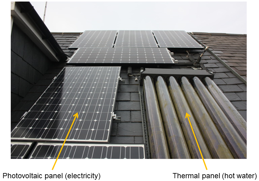
Figure 2. Roof-mounted solar panels

The most dramatic and unusual undertaking to date has been to build a new wall on the outside of the gable-end wall of the house (Figure 3). The purpose of this was to create an insulated cavity. I decided to have it magnificently well-insulated, since the insulation itself is cheap compared with the cost of the work. I’m very pleased with it. Most people don’t notice it in daylight, because the bricks are a good match in colour, but you can see its effect in a thermal image (Figure 4) comparing my house with my neighbours’ on a cold day last winter. The side-wall of my house (on the left) is much colder than theirs, because less heat is leaking through it. The new wall has reduced the gas consumption by more than a third (it’s the downward step after 2010 in the graph).

Figure 3. Adding a new cavity wall to the existing house

Figure 4. Infrared image of Jonathan’s house side wall and his neighbour’s house side wall, showing the much lower heat loss (lower surface temperature) from the insulated wall (left)

The thermal conductivity of the insulating material (solid foam polyisocyanurate, or PIR) is 0.023 W m-1 °C-1. Hence a layer of thickness 190 mm has a u-value of 0.023/0.19=0.12 W m-2 °C-1, so for instance if the difference between the temperature inside and outside the house is 10 degC, the heat flux through the insulator is 1.2 W m-2. I don’t exactly know the thermal conductivity for the old bricks, but it’s probably over ten times greater than for PIR. It’s generally assumed that a traditional solid brick wall, two bricks or nine inches thick, has u of about 2 W m-2 °C-1. Thus, with the addition of the insulator, the side-wall of the house conducts between ten and twenty times less heat than before.

SuperHomes are old houses which have been refurbished by their present owners to reduce their carbon dioxide emissions by at least 60%. The SuperHomes scheme has a register of over 200 such properties. The aim of the scheme is to provide information about refurbishment for energy efficiency, through holding open days in SuperHomes each September. In August 2012, my house qualified as a SuperHome, but there’s still plenty more to be done!

Posted in Climate, Greenhouse gases | Tagged | Leave a comment

Heat waves of the past decade in Chinese mega-cities: a quick review

By Ting Sun

Although cities are often already warmer than their rural surroundings (the well-known “urban heat island” effect), heat waves (HWs), excessively hot periods, will not only enhance the urban and rural temperatures but also exacerbate the contrast between them (Li et al 2015), leading to aggravated thermal stress on urban dwellers (Sun et al 2016). I spent this summer in Beijing and experienced several sultry days in July, which, again, provided me with more sensible HWs than those HW papers I’ve been working on. As September came, Beijing began to cool down; this reminds me of the very cool summer in Reading last year (at least to me). So it seems a good time for a quick review of HWs in Chinese mega-cities of the past decade (2007–2017).

The megacities examined here are those with population larger than 5 million (MoHURD of China, 2016); there are 20 of these, with Shanghai, Beijing and Chongqing the top three populous mega-cities. Temperature observations from the Integrated Surface Database (Smith et al 2011) are employed in this work; however, due to the insufficient data continuity (i.e., consistent records shorter than 30 yrs), two cities (Hong Kong and Shenzhen) are excluded. As such, the following review is only for 18 Chinese mega-cities.  

First, let’s look back at the highest temperatures experienced by these cities during the past summer (Figure 1). Unsurprisingly, records over 35 °C (high temperature according to the Chinese Meteorological Administration, CMA) were recorded at all sites (except for Nanjing, very suspicious records here!) even with highs over 40 °C for several of them.


Figure 1. Daily maximum temperature of 18 Chinese mega-cities recorded during the 2017 summer months (JJA).

Then we move on to the HWs. Although CMA define a period with three or more consecutive days with daily maximum temperature (Tmax) over 35 °C as a HW event, given China is vast country with diverse climates, a location-specific approach (Meehl and Tebaldi 2004) is adopted here for HW identification. With T1 the 97.5th percentile of the observed  series and T2 the 81st percentile, a HW is defined as the longest period that satisfies the following conditions: (1) Tmax > T1 for at least 3 days; (2)   for the entire period; and (3) Tmax > T2 for the entire period, where Tmaxbar denotes the average of Tmax over the HW period.

A total of 973 HWs occurred during the past decade in the 18 mega-cities (Figure 2); in  2009, 2010 and 2017 all the 18 cities experienced HWs. Also, Hefei, Kunming, Changchun, Harbin, Hangzhou and Wuhan experienced HWs all the way through the past ten years, followed by Xi’an, Chengdu, Nanjing, Beijing and Shanghai that recorded HWs in nine of the ten years.

Figure 2. Occurrence of HWs (denoted by empty dots) of 18 Chinese mega-cities between 2007 and 2017.

By looking into the annual HW characteristics, we find more interesting facts. Regarding the annual frequency (i.e. number of HWs per year, Figure 3), 2009, 2010 and the very recent 2017 generally observed more HW events compared with other years. And, solely based on the trend, 2017, similar as 2009, looks to be on an upslope to more HWs.

Figure 3. Annual HW frequency of 18 Chinese mega-cities between 2007 and 2017.

The facts revealed by annual HW durations (i.e., number of HW days per year, Figure 4) are more striking. In addition to 2010 and 2017, 2013 emerges as another “significant” year; this is particularly true to me: I was in Zhejiang that year for the whole summer and underwent highs of 40 °C almost every day! By comparison with the HW frequency, it is clearly shown that HWs of 2013 were even stronger than those of 2010: though with fewer events, HWs persisted longer in 2013. Furthermore, 2017 outperformed other years with the most HW days.

Figure 4. Annual HW duration of 18 Chinese mega-cities between 2007 and 2017.

Following the successive warmest 2015 and 2016 since modern record keeping began in 1880, will 2017 hit a new record? Although an answer to it is not clear yet, this quick review (a far from a thorough investigation) highlights 2017 for the Chinese mega-cities as a remarkable year with the most annual HW days in the past decade. And, if such trend continues, it looks we will “welcome” more HW days in the coming years.

References

MoHURD of China, 2016 Facts of urban development in China: accessed 8 September 2017

Li D, Sun T, Liu M, Yang L, Wang L and Gao Z, 2015. Contrasting responses of urban and rural surface energy budgets to heat waves explain synergies between urban heat islands and heat waves. Environ Res Lett., 10, 054009. doi:10.1088/1748-9326/10/5/054009

Meehl G A and Tebaldi C, 2004. More Intense, More Frequent, and Longer Lasting Heat Waves in the 21st Century. Science, 305, 994–7. DOI: 10.1126/science.1098704

Smith A, Lott N and Vose R, 2011. The integrated surface database: Recent developments and partnerships. Bulletin of the American Meteorological Society, 92, 704–8. https://doi.org/10.1175/2011BAMS3015.1

Sun T, Grimmond C S B and Ni G-H, 2016. How do green roofs mitigate urban thermal stress under heat waves? J Geophys Res-Atmos, 121, 5320–35. https://doi.org/10.1002/2016JD024873

Posted in China, Climate, Climate change, Environmental hazards, Waves | Tagged | Leave a comment

Abrupt climate change at the Royal Meteorological Society

By Joy Singarayer

Recently I was excited to be invited to attend and talk at a Royal Meteorological Society meeting in London on abrupt climate change since the last ice age. The scope of the meeting was to highlight mechanisms driving rapid environmental change during the last 21,000 years, the techniques used to quantify these (there are no direct observations from thousands of years ago, of course), and to discuss the implications for how the climate may evolve in the future. With the palaeo focus being perhaps a bit left field for the Society, we were pleased to find that the meeting was fully booked well in advance, and that the audience, like the speakers, had a good balance of both genders and early-career/established scientists.

At the last glacial maximum, around 21,000 years ago, global average temperature was lower by around 5 degrees Celsius, and sea levels lower by some 120 m, due to the expansion of continental ice-sheets. The process of deglaciation to reach the warm conditions similar to today took roughly ten thousand years, which seems orders of magnitude slower than future anthropogenic climate change projections. However, this process did not occur steadily and monotonically, but was punctuated by several rapid climate change episodes (see Figure 1), just as the last glacial period was.

Figure 1. Screenshot from Liz Thomas’ talk. NGRIP ice core oxygen isotope record for the last 40,000 years. Rapid warming of the Bolling-Alleröd is highlighted and the slower Younger Dryas cooling. MWP-1A and MWP-1B are ice-sheet Melt Water Pulse inputs into the global ocean.

How rapid were some of those changes? Liz Thomas from the British Antarctic Survey reviewed records obtained from ice cores. In some cores (e.g. Greenland North GRIP core) it has been possible to count annual layers within the ice, providing extremely high resolution and accurately dated information. The ratio of different oxygen isotopes (δ18O) in the ice water tells us about the temperature over the ice core region and shows that during the Bolling-Allerod warm transition around 14.7 kyr ago temperatures over Greenland increased by around 10 degrees Celsius in only 1-3 years. Dust contained in the layers originates primarily from low latitude deserts and suggests strongly that changes to low latitude atmospheric circulation and the hydrological cycle preceded the high latitude temperature rise. 

These rapid warmings were likely triggered by strengthening of the Atlantic Ocean overturning circulation. Further talks at the meeting examined these mechanisms through modelling (Lauran Gregoire) and ocean palaeoarchives (Andrea Burke), as well as exploring the impacts on early human societies (William Davies), and then to considering changes during the Holocene interglacial and the impacts of early civilisations, making a bridge to discussion of future anthropogenic change. In the final discussion (Figure 2), led by Paul Valdes, it was noted that while there is no true past analogue to future projected changes, and the mechanisms are different, some of the palaeoclimate changes were of similar magnitudes and speeds to future projections. In this sense they provide useful case studies for model evaluation and for understanding the potential responses of ecosystems to rapid change. They also suggest the importance of Earth System interactions (biosphere, cryosphere, atmospheric chemistry) in producing rapid changes – interactions that are now being more fully incorporated into those climate models being used to simulate future projections of climate change.

Figure 2. The panel discussion at the conclusion of the recent Royal Meteorological Society’s meeting on rapid climate change.

The meeting was organised by Ruza Ivanovic (University of Leeds) and chaired by Prof. Dame Jane Francis (British Antarctic Survey). The presentations (including recordings) and further details about the meeting may be found at the Royal Meteorological Society’s events page.


Posted in Climate, Climate change, Climate modelling, Conferences, Royal Meteorological Society | Leave a comment

The Undergraduate Research Opportunities Programme (UROP)

By Charlie Williams

The Undergraduate Research Opportunities Programme (UROP) is a scheme run by Careers at the University of Reading, enabling undergraduate students in the middle of their degree to work alongside an academic and gain hands-on research experience. They typically work for 6 weeks during the summer, although part-time options are available, and are paid a reasonable salary financed by the University. They are, essentially, a paid intern, working alongside a supervisor and assisting them on a given research project; the supervisor is responsible for writing the proposal, which is then assessed by Careers and funded if deemed appropriate.

Despite the scheme running since 2006, this was the first year I applied to UROP. My proposal was accepted, intended to look at the West African Monsoon (WAM) and how its behaviour has changed in the geological past, present and future. The primary research question was, in its simplest form: Can we use the past to shed any light on the future? This was designed to complement existing research, as part of the much larger PACMEDY project involving several members of the Department and many other institutions.

Research into WAM variability is of great importance, as West African societies are heavily reliant on rain-fed agriculture. Failure, or even just a weakening, of the monsoon can have devastating impacts such as drought, crop failure, famine and other resulting socio-economic issues. Under most scenarios of future climate change, it is believed that the WAM may provide more extreme heavy rainfall events, whilst at the same time becoming more erratic (Biasutti et al. 2008; Diallo et al. 2016). However, there is high uncertainty with many studies disagreeing as to even the sign of change of the WAM, let alone its magnitude or intensity, so one way of assessing our climate models’ projections is to look into the geological past, when analogous climate conditions existed. One example of this is the Mid-Holocene (MH), roughly 6000 years ago, when the WAM was significantly more intense and spatially more extensive, due to a different orbital configuration (Gaetani et al. 2017). This can be seen in Figure 1, where a stronger monsoon extending across West Africa is shown , with a reduction in mean rainfall along the Guinean coast.

Figure 1: Annual mean JJA rainfall differences between the MH and the pre-industrial era, as simulated by the UK Met Office Hadley Centre’s climate model, HadGEM2-ES

The project, therefore, was to compare the behaviour of the WAM over three separate climate states, something currently lacking within the scientific community. Over the summer, my intern and I worked together, focusing in particular on a reasonably well understood physical process within the WAM, namely the West African dipole; this is one of the main patterns of rainfall variability across West Africa, and is characterised by positive (negative) rainfall anomalies over the Sahel and negative (positive) rainfall anomalies along the Guinean coast, associated with negative (positive) SST anomalies in the Gulf of Guinea and equatorial eastern Atlantic (Lough 1986; Janowiak 1988; Cook & Vizy 2006). Several interesting results were found, and although the questions were not entirely resolved within the duration of the UROP placement, sufficient progress was made such that the findings are now being written up for publication.

There are numerous benefits to UROP, both for the student and for the supervisor. For the student, they will hopefully gain many transferable skills, interact with the research community and learn what it is like to be an academic. If the student is interested in a career in research, or is just contemplating postgraduate studies, it provides them with a taster of what full-time research can be like. For the supervisor, it allows an extra ‘pair of hands’ to join your team, for example by conducting research to aid and supplement your existing research or by allowing a pilot project to run. Personally, I found it a very rewarding experience, and very much hope to get a decent paper out of the project – with my intern as co-author, of course!

Acknowledgements

The primary acknowledgement, naturally, goes to my UROP student, Hana E. Beckwith. Secondly, of course, very many thanks to UROP and Careers for funding this project – details of the scheme at http://www.reading.ac.uk/internal/urop/urop_home.aspx

References

Biasutti, M., Held, I. M., Sobel, A. H. & Gianni, A., 2008. SST Forcings and Sahel Rainfall Variability in Simulations of the Twentieth and Twenty-First Centuries. J Clim. 21 (14): 3471-3486

Cook, K. H. & Vizy, E. K., 2006. Coupled Model Simulations of the West African Monsoon System: Twentieth- and Twenty-First-Century Simulations. J Clim. 19: 3681-3703

Diallo, I. et al., 2016. Projected changes of summer monsoon extremes and hydroclimatic regimes over West Africa for the twenty‐first century. Clim Dyn. 47: 3931-3954

Gaetani, M. et al., 2017. West African monsoon dynamics and precipitation: the competition between global SST warming and CO2 increase in CMIP5 idealized simulations. Clim Dyn. 48: 1353-1373

Janowiak, J. E., 1988. An investigation of interannual rainfall variability in Africa. J Clim. 1: 240-255

Lough, M. J., 1986. Tropical Atlantic sea surface temperatures and rainfall variations in sub-Saharan Africa. Mon Wea Rev. 114: 561-570


Posted in Climate, Climate change, Climate modelling, Monsoons, University of Reading | Tagged | Leave a comment

Simulating the effect of electrical charge on cloud drops using Direct Numerical Simulation

By Torsten Auerswald

In the atmosphere, clouds develop when water vapour condenses leading to the formation of cloud drops. This process is usually supported by the presence of condensation nuclei which allow drop formation at low supersaturations. Aerosol particles in the air can act as such condensation nuclei. Once the formation of cloud drops is initiated, several physical processes lead to a growth of the drops. Small drops mainly grow by condensation of water vapour from the surrounding atmosphere onto the drop, while for larger drops collision and subsequent coalescence of drops are the main mechanism for growth.

The collision process of these larger drops is influenced by the size of the drops, as larger drops fall faster than smaller ones. Therefore, larger drops can collect smaller drops due to different terminal velocities. Another important driver for drop collision is turbulence which can lead to an increase in collisions due to the inertia of the drops.

However, not every drop collision results in coalescence. Two colliding drops can bounce off from each other or break up into smaller drops. It can be shown that successful coalescence is more likely when the colliding drops are electrically charged. Charging of drops can occur naturally due to background radioactivity and cosmic rays, which form ions in the atmosphere and cause aerosol particles to carry a slight charge. Thus, by charged aerosol particles acting as condensation nuclei, charged cloud drops are formed. Because of the polarisation of one drop from the charge carried by another drop, even drops with like charges will experience attractive forces, given that their separation distance is sufficiently small. This effect increases the efficiency of the collision and coalescence processes in the cloud and therefore can act to accelerate the drop growth and ultimately the production of raindrops.

In our project we are developing a model to simulate the behaviour of cloud drops in a warm cloud. For a small volume of such a cloud the turbulent flow is simulated using Direct Numerical Simulation (DNS) and the collision of drops in the turbulent flow is studied. By introducing charged drops into the simulation and considering the electrical forces resulting from the charge, we will be able to investigate the influence of electrical charge on the collision rate and size distribution of cloud drops and the production of rain drops.

To illustrate this type of simulation, the figure below shows a snapshot from a simulation where cloud drops are moving in a flow with periodic boundary conditions and growing by collision.To see the animation click on this link.

Posted in Aerosols, Climate | Tagged | Leave a comment

Forecasting the Indian monsoon

By Arathy Menon

The South Asian monsoon, which brings rainfall to India and the neighbouring countries during the boreal summer season, is a major atmospheric circulation system. India receives more than 80% of its annual rainfall during the monsoon season, generally occurring from June to September. However, the monsoon onset can also occur as early as May and the withdrawal can occur as late as early October, while the season itself is comprised of several wet and dry periods which occur as a part of the intraseasonal variability. Any variability in the timing, duration and intensity of the monsoon can have a significant impact on rain-fed agriculture that contributes a major portion of India’s GDP.  Irrespective of recent growth in service and industrial sectors, agriculture is still the predominant occupation in many rural regions of India. The Indian monsoon also has significant impact on the coal and steel industries, thereby affecting the world economy. Hence understanding and predicting the monsoon is vital.

The forecasting centres around the world try to predict the monsoon onset and amount at least a season in advance. However, it is notoriously difficult to predict the timing of the onset as well as the overall seasonal rainfall. The models participating in the latest version of the Coupled Model Intercomparison Project showed considerable improvement in simulating the mean rainfall and variability of the South Asian monsoon compared to earlier models; however, a dry bias still exists over India in most of these models (Sperber et al., 2013). The ability to predict the monsoon at least a season in advance is limited as it is difficult to represent tropical convection (the processes leading to monsoon rainfall) in our forecast models, and we lack a proper understanding of the way in which land and ocean surfaces alter the atmosphere on small scales to initiate monsoon storms. Hence detailed observations of the lower layers of the atmosphere and surface are needed to understand such processes.

In order to achieve this, an intensive field campaign was conducted in India during summer 2016 as part of the INCOMPASS project (refer to Dr Andrew Turner’s blog for more detail). During summer 2016, we took the UK’s Atmospheric Research Aircraft (operated by the Facility for Airborne Atmospheric Measurement), a modified BAe 146, on its first-ever mission to India to gather new monsoon observations (Figure 1). The flight observations were accompanied by ground-based observations from towers that measure the surface temperature, soil conditions and fluxes of temperature and moisture into the atmosphere as well as weather balloons which were launched from a network of weather stations spread over India. We are now using the data collected to challenge and improve our forecast models, at the UK Met Office and India’s National Centre for Medium Range Weather Forecasting.

Figure 1. The FAAM atmospheric research aircraft, a modified BAe 146

Climate models generally have a coarse spatial resolution, which means that atmospheric and oceanic processes operating at a smaller scale (for example convective precipitation) cannot be predicted by physical equations but instead we have to resort to a process called parametrization. This will help us to represent the effects of finer scale processes such as clouds on the coarser scale meteorology. Due to this inadequacy, climate models when used to simulate the monsoon cannot capture many important features of the monsoon. The most effective way of solving this problem is to use a model with finer resolution (grid spacing). The Met Office Unified Model (MetUM – Brown et al., 2012) uses the same dynamics and physics both at numerical weather prediction and climate projection scales. Hence it is a perfect tool to better understand the physical mechanisms involved in monsoon rainfall and to determine the role of model resolution in improving monsoon forecasts.  

For our use, we have customized the MetUM with a ‘nested suite’, which is a fine-scale regional model placed inside a coarser resolution global model. Using this method, we can operate a very fine resolution (4 km grid spacing) model for South Asia and outside this ‘nest’ the model will have coarser grid resolution (~17 km over the rest of the globe). The 4 km grid-spacing is common for forecasts in the UK but is more computationally challenging for a country the size of India. Figure 2 shows the impact of the grid spacing on forecasts of monsoon rainfall during 2016.  It features a monsoon depression, a low-pressure system, that formed in the Bay of Bengal during early July 2016 and shows that it is captured well by the models. However, the details of the clouds and rainfall are much finer. The individual convective cells are apparent in the finer resolution version of the model. This type of monsoon storm is often implicated in heavy monsoon rains and flooding, such as the recent events of August 2017 in Mumbai.


Figure 2. Rainfall rate (shaded), snowfall rate (shaded), total cloud fraction (shaded) and mean sea level pressure (contours) from 4 km resolution model (left) and global model (right) on 7 July 2016. An animation for the period 1 to 7 July 2016 is available via this link: http://www.met.reading.ac.uk/~xr911612/home/anims.gif. In the animation, spiral bands of rainfall associated with the monsoon depression are seen over eastern parts of India on 6th and 7th July.

Currently, we are running two experiments for the 2016 monsoon with this setup contrasting them by using different land surface conditions such as soil moisture and vegetation types, which will eventually improve our understanding of the impact of changing land-surface conditions on monsoon rains. As the project continues we will pioneer development of even-finer resolution models, down to 100 m scales, which will allow us to examine storm development and frontal weather system structures with high fidelity.

By improved theoretical understanding of the physical processes of the monsoon and an improvement in rainfall prediction, the work will allow improved agricultural planning and security of the food supply, benefiting the Indian economy.

References

Brown, A., Milton, S., Cullen, M., Golding, B., Mitchell, J., & Shelly, A., 2012. Unified modeling and prediction of weather and climate: A 25-year journey. Bulletin of the American Meteorological Society,  93(12): 1865-1877.

Sperber, K. R., Annamalai, H., Kang, I. S., Kitoh, A., Moise, A., Turner, A., Wang, B., & Zhou, T., 2013. The Asian summer monsoon: an intercomparison of CMIP5 vs. CMIP3 simulations of the late 20th century. Climate Dynamics, 41(9-10), 2711-2744.

Posted in Climate, Climate modelling, Monsoons, Numerical modelling, Seasonal forecasting | Leave a comment

Recent progress on decadal prediction in the North Atlantic

by Jon Robson

The North Atlantic is a region of the Earth that is characterised by pronounced multi-decadal variability in surface temperatures – a phenomenon that has become known as Atlantic Multi-decadal Variability (AMV, see Sutton et al for a short review). The North Atlantic also appears to be one of the most predictable areas on Earth, with surface temperature and ocean heat content in the subpolar North Atlantic (~50-70°N) apparently predictable up to a decade in advance. This is encouraging given that AMV has also been associated with considerable societal impacts, including modulating the number of Atlantic hurricanes and rainfall over the Sahel (see Figure 1f and 1g).

Figure 1. An overview of Atlantic Multi-decadal Variability (AMV). (a) shows sea surface temperature anomalies for global (blue) and Atlantic (red) and the resulting AMV index (black). (b) and (c) shows proxies of ocean strength in the North Atlantic and sulphate aerosol precursor emissions. (d) shows the spatial extent of the AMV pattern. (e), (f) and (g) shows variability in winter time North Atlantic Oscillation, Hurricane accumulated energy and Sahel Rainfall. Thick lines show 10 year running means.

We recently argued that the high level of predictability of subpolar North Atlantic temperature is consistent with the initialisation of – but not necessarily the prediction of – the thermohaline component of the ocean circulation. Put another way, hindcasts appear skillfully to predict large changes in temperature only when they are started from an anomalous ocean circulation, rather than being able to predict the onset of an anomalous ocean circulation itself. Nevertheless, it is the slow evolution of the anomalous ocean circulation which allows us to predict North Atlantic upper-ocean temperature in advance. The prediction of upper-ocean temperatures can also lead to skillful predictions of other variables; for example, recent advances in 2-5 year predictions of Sahel rainfall and summer surface temperature over China are both related to improved predictions of the North Atlantic.

The particular view of the slow changes in the North Atlantic being governed by slow changes in the thermohaline circulation hasn’t really moved on from the main paradigms of the early 2000s. However, there have been a number of challenges to this view. In particular, multi-decadal changes in regional forcings (particularly Anthropogenic Sulphate Aerosols), or local thermodynamic coupling of the atmospheric variability, have both been proposed to be the main controlling factor of AMV. Long-story-short, we know that many models’ simulation of the Atlantic and AMV is deficient when compared to observations, and the role of the external forcing, in particular, is a major uncertainty. For decadal predictions, the forcings certainly provide skill, particularly in the tropical Atlantic. However, apart from the long-term warming trend, little is known about the role of different forcing factors (e.g. volcanic or anthropogenic aerosols, or solar), nor do we understand how the forcings are leading to skill, or even if the forced responses are realistic.

So where will progress come from over the next few years? Well, interesting changes abound in the North Atlantic at the moment. The subpolar North Atlantic may be transitioning into a cold state similar to that last observed in the 1970s-1980s (see Figure 2), and many people (including yours truly) have published tentative predictions of a further cooling of the North Atlantic. The Atlantic is also now observed at unprecedented levels of detail (for example the RAPID and OSNAP programs), so these changes will be watched closely.

Figure 2. 0-700 m heat content anomalies in the North Atlantic subpolar gyre region computed from the NODC data set. Figure created using KNMI climate explorer.

On the modelling side, recent advances in predicting the North Atlantic Oscillation on multi-year timescales could open the doors to further Atlantic-wide improvements. Near-term Climate Prediction is also now a World Climate Research Program “Grand Challenge”. Finally, international modelling experiments like the Decadal Climate Prediction Project (DCPP, a CMIP6 endorsed MIP) will continue the exploration of “near-term” climate prediction. DCPP will also further co-ordinate the real-time decadal prediction efforts of the community, as well as more process focused sensitivity studies. More generally, the wider CMIP6 activities (from highResMIP to VolMIP) also offer new opportunities.

Finally, the UK ACSIS project  is beginning better to co-ordinate and integrate the UK’s scientific expertise in observations and modelling across atmosphere (including composition), ocean and cryosphere, in order to tackle the multi-faceted, multi-disciplinary problem of understanding multi-decadal timescale variability in the North Atlantic.

So, taken altogether, there is a lot of North Atlantic Science to look forward to; I just wish I could find the time to look at all the things I want to!

References

Sutton, R. T., McCarthy, G. D., Robson, J., Sinha, B., Archibald, A. and Gray, L. J., 2017. Atlantic Multi-decadal Variability and the UK ACSIS Programme. Bulletin of the American Meteorological Society. ISSN 1520-0477 doi: 10.1175/BAMS-D-16-0266.1

Yeager, S. G. and Robson, J. I., 2017. Recent progress in understanding and predicting Atlantic decadal climate variability. Current Climate Change Reports, 3 (2). pp. 112-127. ISSN 2198-6061 doi: 10.1007/s40641-017-0064-z

Monerie, PA., Robson, J., Dong, B. et al., 2017. A role of the Atlantic Ocean in predicting summer surface air temperature over North East Asia? Climate Dynamics. doi: 10.1007/s00382-017-3935-z

Robson, J., Polo, I., Hodson, D. L. R., Stevens, D. P. and Shaffrey, L. C., 2017. Decadal prediction of the North Atlantic subpolar gyre in the HiGEM high-resolution climate model. Climate Dynamics. ISSN 0930-7575 doi: 10.1007/s00382-017-3649-2

Sheen et al, 2017. Skilful prediction of Sahel summer rainfall on inter-annual and multi-year timescales, Nature Communications 8, doi: 10.1038/ncomms14966

Dunstone N, Smith D, Scaife A, Hermanson L, Eade R, Robinson N, Andrews M, Knight J., 2016. Skilful predictions of the winter North Atlantic oscillation one year ahead. Nat Geosci 9:809–814. doi:10.1038/ngeo2824

Posted in Climate, Climate change, Climate modelling, Oceans | Tagged | Leave a comment

Without the Tibetan Plateau, what would happen to the Asian summer monsoons?

By Mike Wong

The Tibetan Plateau is the highest and most extensive plateau in the world, with an average elevation exceeding 4000 metres and stretching over 2.5 million square kilometres. While it is often called the ‘rooftop of the world’, it also serves as the ‘water tower of the world’. Many major rivers in Asia, including the Yangtze, Mekong and the Ganges, originate from the Tibetan Plateau and support the livelihoods of more than 40% of the world’s population living in rapidly developing economies such as China and India.

The Tibetan Plateau is also a crucial component of the Asian climate. During late spring to early summer, its vast and elevated surface heats up rapidly and acts as a highly effective heat source for the atmosphere above. The heating from the plateau’s surface is long believed to be vital in creating ascent and supporting the meridional overturning circulation of the Indian Summer Monsoon.

However, recent studies (e.g. Boos and Kuang 2010, 2013, Wu et al. 2012) questioned the impact of the Tibetan Plateau on the Indian summer monsoon. Using idealised orography in which the Tibetan Plateau is removed, keeping only the Himalayas, these studies demonstrated that the Indian summer monsoon can be maintained in global climate model simulations. Therefore, the current consensus in the literature is that the orographic sheltering provided by the Himalayas is equally important, or perhaps more important, than the elevated surface heating from the Tibetan Plateau in maintaining the Indian summer monsoon.

Funded by the Climate Science for Service Partnership China (CSSP-China), the MESETA project aims to investigate further the role of the Tibetan Plateau in maintaining the Asian summer monsoons. Following previous studies, the Met Office’s global climate model HadGEM3 is used to perform various simulation experiments with idealised orography. Three different modifications to the orography are used to demonstrate the impact of the Tibetan Plateau, Himalayas and the Iranian Plateau on the Asian monsoons (Figure 1a-d). The simulations are performed at N96 resolution (200 km grid spacing at the equator) covering the period between 1981 and 2001, providing 20 years’ worth of data to derive the climatology of the summer monsoons. First, a control experiment is performed using the default orography and Figure 2a shows the summer (June-August) average precipitation and 850 hPa wind. Results from each sensitivity experiment is then compared to the control.

Figure 1. Surface orography used in each experiment:  a) Control; b) No Tibetan Plateau; c) Himalayas and Iranian Plateau only and d) Himalayas only.

The first experiment, No Tibetan Plateau (Figure 2b-c), focuses on the impact of the Tibetan Plateau and Himalayas on the monsoons by removing both terrains from the model. Compared to the control experiment, the Indian summer monsoon clearly weakened as indicated by the easterly anomalies over the Arabian Sea. Although there is more rainfall over India compared to the control, it is mostly likely related to HadGEM3’s bias in simulating summer rainfall in the region. There is also a reduction in rainfall over most of China, suggesting a weakened East Asian summer monsoon. Therefore, this experiment shows that without the Tibetan Plateau and the Himalayas, both the Indian summer monsoon and the East Asian summer monsoon will be a lot weaker in intensity.

Figure 2. Summer precipitation and 850 hPa wind (left column) and difference relative to control : a) Control; b-c) No Tibetan Plateau; d-e) Himalayas and Iranian Plateau only; f-g) Himalayas only.

However, things improved greatly in the second experiment when the Himalayas were put back into the model (Himalayas and Iranian Plateau only, Figure 2 d-e). Low level circulation over the Arabian Sea and India is more consistent to the control as the easterly anomalies reduced, while summer rainfall over India is also more similar to the control. Therefore, it seems that the Indian summer monsoon can indeed be maintained even if the elevation of the plateau is drastically reduced as long as the Himalayas are intact. In contrast, the East Asian summer monsoon is more sensitive to the presence of the Plateau as most of China is still receiving less summer rainfall than the control.

While the first two experiments demonstrated the crucial role of the Himalayas, the third experiment, Himalayas only (Figure 2 f-g), focuses on the importance of the Iranian Plateau. In this experiment, the Iranian Plateau is removed leaving only the Himalayan ridges in the model such that their contribution can be isolated. Without the Iranian Plateau, the summer westerlies over the Arabian Sea are weakened and the region is affected by north-easterly wind anomalies, bringing dry continental airmass into the region. Although the weakening of the westerly monsoon is not as significant as in the No Tibetan Plateau experiment, the results here show that the Iranian Plateau also exerts considerable influence on the Indian summer monsoon.

To summarise, the idealised experiments here show that the Indian summer monsoon is not sensitive to the elevation of the Tibetan Plateau as long as the Himalayas and the Iranian Plateau are present. In contrast, the East Asian summer monsoon is more sensitive to the presence of the Tibetan Plateau. Also, it is necessary to consider the impact of model bias as the monsoons in the control experiment are not perfect reconstructions, especially in terms of rainfall. To further examine how much of the results are model dependent, some of the experiments will be repeated in other climate models through the forthcoming Global Monsoon Model Inter-comparison Project (GMMIP). So, if one day the Tibetan Plateau somehow disappeared, don’t worry, the Indian summer monsoon will probably be fine (too bad for East Asian summer monsoon though …).

References

Boos WR and Kuaang Z., 2010. Dominant control of the south Asian monsoon by orographic insulation versus plateau heating. Nature, 463 (7278): 218-222.

Boos WR and Kuang Z., 2013. Sensitivity of the south Asian monsoon to elevated and non-elevated heating. Scientific reports 3.

Wu G, Liu Y, He B, Bao Q, Duan A, Jin FF, 2012. Thermal controls on the Asian summer monsoon. Scientific Reports 2.

Posted in Climate, Climate modelling, Monsoons, Numerical modelling | Leave a comment

Can we use future data to improve our knowledge of the ocean?

By Chris Thomas

An interesting problem in climate science is working out what happened in the world’s oceans in the last century. How did the temperature change, where were the currents strongest, and how much ice was there at the poles? These questions are interesting for many reasons, including the fact that most global warming is thought to be occurring in the oceans and learning more about when and where this happened will be very useful for both scientists and policymakers.

There are several ways to approach the problem. The first, and maybe the most obvious, is to use the observations that were recorded at the time. For example, there are measurements of the sea surface temperature spanning the entire last century. These measurements were made by (e.g.) instruments carried on ships, buoys drifting in the ocean, and (in recent decades) satellites. This approach is the most direct use of the data, and arguably the purest way to determine what really happened. However, particularly in the ocean, the observations can be thinly scattered, and producing a complete global map of temperature requires making various assumptions which may or may not be valid.

The second approach is to use a computer model. State-of-the-art models contain a huge amount of physics and are typically run on supercomputers due to their size and complexity. Models of the ocean and atmosphere can be guided using our knowledge of factors such as the amount of COin the atmosphere and the intensity of solar radiation received by the Earth. Although contemporary climate models have made many successful predictions and are used extensively to study climate phenomena, the precise evolution of an individual model run will not necessarily reproduce reality particularly closely due to the random variation which often occurs.

The final technique is to try to combine the first two approaches in what is known as a reanalysis. The process of reanalysis involves taking observations and combining them with climate models in order to work out what the climate was doing in the past. Large-scale reanalyses usually cover multiple decades of observations. The aim is to build up a consistent picture of the evolution of the climate using observations to modify the evolution of the model in the most optimal way. Reanalyses can yield valuable information about the performance of models (enabling them to be tuned), explore aspects of the climate system which are difficult to observe, explain various observed phenomena, and aid predictions of the future evolution of the climate system. That’s not to say that reanalyses don’t have problems, of course; a common criticism is that various physical parameters are not necessarily conserved (which can happen if the model and observations are radically different). Even so, many meteorological centres around the world have conducted extensive reanalyses of climate data. Examples of recent reanalyses include GloSea5 (Jackson et al. 2016), CERA-20CMERRA-2 (Gelaro et al. (2017)) and JRA-55 (Kobayashi et al. (2015)).

When performing a reanalysis the observations are typically divided into consecutive “windows” spanning a few days. The model starts at the beginning of the first window and runs forward in time. The reanalysis procedure pushes the model trajectory towards any observations that are in each window; the amount by which the model is moved depends on how much we believe the model is correct instead of the observation. A very simplified schematic of the procedure can be found in Figure 1.

Figure 1: A very simplified schematic of how reanalysis works. The data (black stars) are divided into time windows indicated by the vertical lines. The model, if left to its own devices, would take the blue trajectory. If the data are used in conjunction with the model it follows the orange trajectory.

This takes us to the title of the post. Obviously it’s not actually possible to use data from the future (without a convenient time machine), but the nice aspect of a reanalysis is that all of the data are available for the entire run. Towards the start of the run we have knowledge of the observations in the “future”; if we believe these observations will enable us to push the current model closer to reality it is desirable for us to use them as effectively as possible. One way to do that would be to extend the length of the windows, but that eventually becomes computationally unfeasible (even with the incredible supercomputing power available these days).

The question, therefore, is whether we can use data from the “future” to influence the model at the current time, without having to extend the window to unrealistic lengths. The methodology to do this has been introduced in our paper (Thomas and Haines, 2017). The essential idea is to use a two-stage procedure. The first run is a standard reanalysis which incorporates all data except the observations that appear in the future. The second stage then uses the future data to modify the trajectory again. Two stages are required because the key quantity of interest is the offset between the future observations and the first trajectory; without this, we’d just be guessing how the model would behave and would not be able to exploit the observations as effectively.

Our paper describes a test of the method using a simple system: a sine-wave shape travelling around a ring. Observations are generated at different locations and the model trajectory is modified accordingly. It is found that including the future observations improves the description relative to the first stage; some results are shown in Figure 2. The method has been tested in a variety of situations (including different models) and is reasonably robust even when the model varies considerably through time.

Figure 2: Results obtained when using the new methodology in a simple simulation. The left hand plot shows the results after the first stage, and the right hand plot shows the results after the second stage. In each plot the horizontal axis is space and the vertical axis is time. Values closer to zero (the white areas) indicate the procedure has performed well, whereas values further from zero (the blue and orange areas) indicate it has not been as successful. The second stage has more white areas, showing an improvement over the first. (The labels at the top of each plot indicate where the observations are located.)

We have now implemented the method in a large-scale ocean reanalysis which is currently running on a supercomputer. We are particularly interested in a process known as the AMOC (Atlantic Meridional Overturning Circulation) which is a North-South movement of water in the Atlantic Ocean (see Figure 3 for a cartoon). It is believed that the behaviour of water in the northernmost reaches of the Atlantic can influence the strength of circulation in the tropical latitudes; crucially, this relationship is strongest at a time lag of several years (Polo et al. (2014)). Data collected by the RAPID measurement array in the North Atlantic (www.rapid.ac.uk) take the role of the “future” data in the reanalysis and are used to modify the model trajectory in the North Atlantic. The incorporation of RAPID data in this way has not been done before and we’re looking forward to the results!

Figure 3: A cartoon of the AMOC and the RAPID array in the North Atlantic (adapted from www.rapid.ac.uk). The red and blue curves indicate the movement of water. The yellow circles indicate roughly where the RAPID array is located.

References

Jackson, L. C., Peterson, K. A., Roberts, C. D. and Wood, R. A. 2016. Recent slowing of Atlantic overturning circulation as a recovery from earlier strengthening. Nat. Geosci. 9(7), 518–522. http://dx.doi.org/10.1038/ngeo2715

Kobayashi, S. et al. 2015. The JRA-55 Reanalysis: General specifications and basic characteristics. J. Meteor. Soc. Japan Ser. II 93(1), 5–48. http://dx.doi.org/10.2151/jmsj.2015-001

Gelaro, R. et al. 2017. The Modern-Era Retrospective Analysis for Research and Applications, Version 2 (MERRA-2) J. Clim. 30(14), 5419–5454. http://dx.doi.org/10.1175/JCLI-D-16-0758.1

Thomas, C. M. and Haines, K. 2017. Using lagged covariances in data assimilation. Accepted for publication in Tellus Ahttp://dx.doi.org/10.1080/16000870.2017.1377589 

Polo, I., Robson, J., Sutton, R. and Balmaseda, M. A. 2014. The Importance of Wind and Buoyancy Forcing for the Boundary Density Variations and the Geostrophic Component of the AMOC at 26°N. J. Phys. Oceanogr. 44(9), 2387–2408. http://dx.doi.org/10.1175/JPO-D-13-0264.1


Posted in Climate, Climate modelling, Oceans | Tagged | Leave a comment

Sunny, Windy Sundays

By Daniel Drew

Throughout the day National Grid (the system operator of the electricity network in Great Britain) must ensure there is a balance between the demand for electricity and the amount generated. Historically this has involved forecasting the level of demand based on meteorological conditions and human activity and adjusting the generation from conventional power stations accordingly. However, the dramatic growth of wind and solar power capacity in recent years makes things more complicated as there is now a need accurately to forecast the renewable generation as well.

National Grid has a licence obligation to keep the system frequency between 49.5 and 50.5 Hz. Any imbalance between supply and demand leads to a change in the frequency of the network. The rate at which the frequency changes following an imbalance between supply and demand is dependent on the system inertia – higher levels mean it takes longer to reach a new steady state. System inertia is the stored rotating energy of all the machines directly connected to the network, it is therefore a measure of resistance in the network to changes in frequency. The growth of renewable generators such as solar panels and wind turbines reduces the amount of system inertia. This presents a challenge to National Grid, particularly on days where renewables provide a large proportion of demand. It is therefore important to have a clear understanding of the proportion of electricity provided by renewables throughout the year.

During the calendar year of 2016, wind and solar power contributed approximately 15% of UK electricity. However, for individual 30 minute periods this proportion can be a lot higher. Figure 1 shows that the contribution of renewables to electricity demand exceeded 25% for approximately 5% of the year. In general, the highest penetrations are observed on sunny, windy and warm days, when the electricity demand is relatively low and the generation levels of wind and solar are both relatively high. If these meteorological conditions happen to fall on a Sunday the proportion of renewables is amplified as electricity demand is highly suppressed.

Figure 1. The cumulative distribution of the 30 min proportion of electricity demand provided by wind and solar power for 2016. Derived from data from https://www.bmreports.com/.

Given the short time period for which the turbines and solar panels have been installed, the distributions shown in Figure 1 are based on a limited number of meteorological conditions. It is therefore unclear what proportion of demand could be provided by renewables based on the current capacity of wind farms and solar panels. We are therefore currently working with National Grid to extend the dataset taking into account the full range of meteorological conditions which could occur in the UK.


Posted in Renewable energy | Leave a comment