By Dr. Chris Skinner (University of Hull) 9th May 2014

The scientific conference is a vital way for scientists to meet and discuss their research with one another. They are an opportunity both for yourself to share your latest research, and receiving first hand feedback/criticism for it, and to catch up on the latest, and cutting edge research that is going on in other institutions. When it come to conferences, they do not get much bigger than the European Geosciences Union’s General Assembly, affectionately known as EGU.

EGU is an annual, weeklong conference held in Vienna, around Easter time. For many of us working as part of the FFIR programme, it is a vital fixture in our calendars, and that is simply because of its size. It is big, real big. To give you some figures taken from their website, the 2014 meeting was attended by 12,437 scientists from 106 countries, who presented 9,583 posters and gave 4,829 oral presentations. I was but one of 1,120 scientists from the UK. The advantage of it being so big is that a lot of people – important, clever and useful people – attend and they encompass a wide range of disciplines. It is fertile ground for new ideas and collaborations.

A 360° panoramic from outside the EGU (Austria Centre Vienna)

A typical day at EGU is a long one. The oral sessions begin at 8.30am and last for six 15 minute presentations before a half hour coffee break – where one can sample the delights of a Viennese Melange. Two sessions in the morning are followed by an hour and a half break for lunch. This is a chance to grab some food, peruse the several, large poster halls, and have a look around the displays in the foyer. These range from ESA, to representatives from scientific publishers, to companies promoting the equipment or services they have for sale. My personal favourite was from the Earth Engine team from Google, who were demonstrating their beta for an open source GIS – it is one to keep an eye on. After lunch there are a further two oral session blocks until 5.00pm, and these are followed by a two hour poster session where you have the opportunity to talk to the poster’s author. These are always lively and busy. From 7.00pm there are often further things to attend, such as meetings, workshops or debates – my week included a SINATRA team meeting and a function to celebrate the successful first year of the Earth Surface Dynamics open-access journal.

A session I found particularly interesting this year was the “Precipitation: Measurement, Climatology, Remote Sensing, Modelling” session. It featured several presentations regarding the development of the Global Precipitation Measurement mission (GPM), which aims to dramatically increase the coverage of satellite instrumentation that can directly detect rainfall and its relative intensity. The core satellite in the constellation launched earlier in 2014 and from the sessions it is clear that it is working well, and the indicators are that our ability to observe rainfall from orbit will be greatly improved. This might not have a huge impact on forecasting FFIR in the UK, where we are well served by ground recording instrumentation, but will have a big impact on areas that are not, such as South America and sub-Saharan Africa.

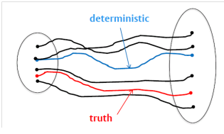
My favourite presentation of the week, however, was given by Massimiliano Zappa, from the Swiss Federal Research Institute. Zappa’s presentation was one of the invited presentations in the “Ensemble hydro-meteorological forecasting” session, titled “HEPS challenges the wisdom of the crowds: the PEAK-Box Game. Try it yourself!”  The PEAK-Box approach is a method of better understanding and communicating the uncertainty around peak flood forecasts, by using a visual box representing the possible range of peak discharges from a forecast ensemble, and during the session Zappa had the audience make their own predictions (a bit like the old ‘Spot the Ball’ competitions). He predicted that, through the “wisdom of the crowd”, the average of the audience’s response should be close to the actual peak flood. I will let you know when he has finished collating and distributing the results whether or not it has worked!

This blog is just a mere flavour of the activities at EGU. For me, personally, the most rewarding and productive aspect is getting to meet, face to face, many of the people I will be working alongside in the SINATRA project, as well as many excellent scientists from around the globe that beforehand I had only ever communicated with on Twitter, or in the blogosphere. And if you get the chance to escape for a few hours, there is always the beautiful city of Vienna to explore.

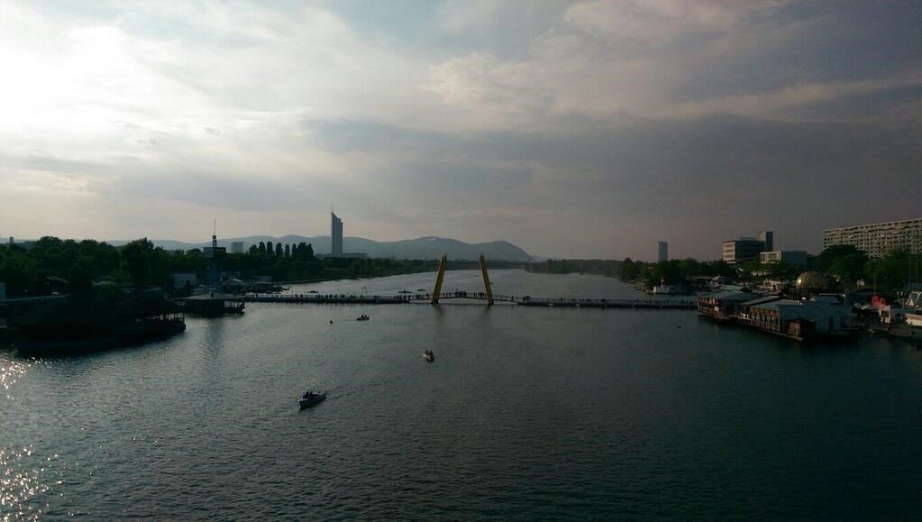
View over the New Danube at sunset, close to EGU. It’s pretty nice.

You can follow Chris Skinner on Twitter: @cloudskinner

By Dr. Laura Baker (University of Reading) 14th April 2014

Ensemble weather forecasts are used to represent the uncertainty in the forecast, rather than just giving a single deterministic forecast. In a very predictable system, all the ensemble members typically follow a similar path, while in an unpredictable system, the ensemble may have a large divergence or spread between members.

Schematic diagram of an ensemble system

A simple way to create an ensemble is to perturb the initial conditions of the forecast. Since the atmosphere is a chaotic system, a small perturbation can potentially lead to a large difference in the forecast. However, just perturbing the initial conditions of the forecast is sometimes not enough, and these ensembles can often be underspread, which means that they do not cover the full range of possible states that could occur. This means that the ensemble forecast could miss what actually occurs in observations. One way to further increase the spread of the ensemble is to add some representation of model error, or model uncertainty, into the forecast. Model uncertainty becomes relatively more important as you go down to smaller scales, so in a high-resolution ensemble it is more important to include these effects.

A recent study as part of the DIAMET project (http://www.ncas.ac.uk/index.php/en/diamet-introduction) aimed to investigate the effects of randomly perturbing individual parameters in the forecast model as a way of representing model error. We used a configuration of the Met Office Unified Model with a resolution of 1.5 km and a domain covering the southern part of the UK. We generated an ensemble with one control member and 23 perturbed members. The initial conditions for each ensemble member came from a global ensemble forecast with a lower resolution (60 km). Since our domain is a sub-domain of the global model, the lateral boundary conditions are also derived from the global model forecast, and each ensemble member has perturbed boundary conditions corresponding to their initial condition perturbations.

We focussed on a single case study which occurred during one of the DIAMET field campaign periods. This case was particularly interesting from an ensembles perspective because it involved the passage of a frontal rain band with an interesting banded structure which was not well represented in the operational forecast. None of the individual ensemble members captured the two separate rain bands, but some of them had rain in the location of the second band.

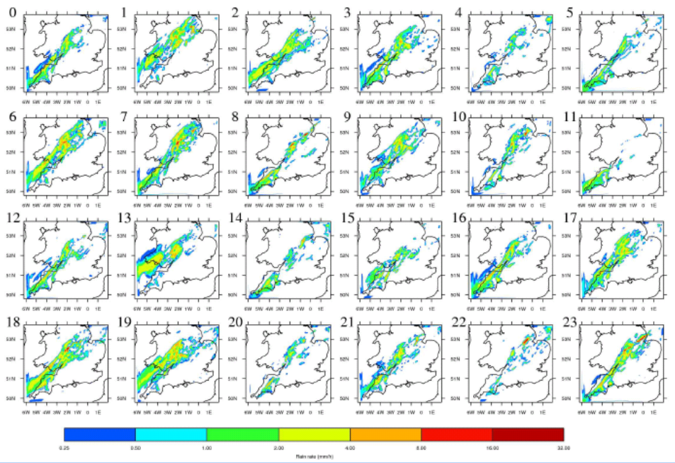
The left panel shows the radar rain rate at 1500 UTC on 20 September 2011. The right panel shows the control member forecast rain rate at the same time. The model fails to capture the second rain band.

This figure shows each of the ensemble members in the ensemble (before the parameter perturbations were applied) at the same time as the figure above. Note the large variability in the position and intensity of the rain band between members.

We perturbed parameters in the boundary layer and microphysics parameterisation schemes. 16 parameters were chosen to be perturbed, which were known by experts to have some uncertainty in their values. We perturbed each parameter randomly within a certain range, and each ensemble member had different random perturbations applied to its parameters. We focussed our analysis on near-surface variables (wind speed, temperature and relative humidity) which could be compared with observations from surface stations, and rainfall rate and accumulation (which could be compared with radar observations). We found that for the near-surface variables, representing model error using this method improved the forecast skill and increased the spread of the ensemble. In contrast, for the rainfall the forecast skill and ensemble spread were degraded by this method after the first couple of hours of the forecast.

This study is a useful first step to developing a high-resolution ensemble system with a representation of model error. This work was recently published in Nonlinear Processes in Geophysics and can be accessed here: http://www.nonlin-processes-geophys.net/21/19/2014/npg-21-19-2014.html .

By Dr. Rob Thompson (University of Reading) 4th April 2014

If we are looking to predict flooding from intense rainfall, we are going to need to know just how intense that rainfall really is – and where. The traditional way to measure rainfall is with a raingauge – a collector that measures the amount of rain falling into a collector of area around 50 square cm. Of course a raingauge can only measure the rainfall at the site, for areal coverage, we turn to radar.

Weather radar developed after the second world war when weather echoes had been noticed in aircraft and ship tracking radars. They developed until the 1980s when weather radar networks were being built, including in the UK. The (slightly out of date) Met Office fact sheet 15 provides an excellent explanation of how weather radar works and the addition of Doppler radar (which is something of a misnomer, it in fact does not use the Doppler shift, the effect would be too small to measure) so I won’t be repeating that. I shall instead be discussing the latest development in the UK network and one that is currently rolling out is dual-polarisation (at the time of writing there are 4 dual-polarisation radars in the UK network).

Doppler Radar Weather Station, Thurnham (1) (Danny Robinson) / CC BY-SA 2.0

What is Dual-Polarisation?

So what is dual polarisation and what does it give us? With a modern dual polarisation radar the radar considers horizontally and vertically polarised waves separately. Usually they are transmitted simultaneously and the received and separated. This leads to a range of new parameters that are of use to the radar meteorologist and therefore is of great benefit. Those benefits are only now being fully researched (including in the FRANC project by me) but include improved rejection of non-meteorological echoes, better classification of echoes (detecting rain/snow/hail etc.) and importantly, improved ability to quantitatively measure in heavy rain.

Using Radar in Intense Rainfall

During very heavy rainfall, some of the electromagnetic waves from the radar are absorbed or scattered out of the beam (that proportion of the scattering back to the radar is the radar signal), that means that there is less power in the beam beyond the rain. When rain is very heavy this can result in the beam having significantly reduced power from returns beyond heavy rain and therefore appears to show less rainfall than is truly there.

The figure shows the reflectivity of very intense rainfall event passing London on 20th July 2007. Warmer colours show high reflectivities and hence heavier rainfall. The radar is the star on the right side of the image, and it is clear to see that there is a “hole” in the radar echo behind the intense band of rainfall. This appears as a “searchlight”, and at it’s worst when the intense rain band lines up with the radar for maximal absorption of the radar beam. This particularly extreme case is also labelled with how serious the problem is, without knowledge of this “attenuation” problem, only 4mm/hr rainfall would be observed for Heathrow, when gauged measurement suggested that was 68mm/hr. Without dual-polarisation capability, a conventional radar can estimate the attenuation, but this estimate is unstable and so cannot be used to make large corrections such as required in a case like this as it could introduce greater errors than it fixed. That means that with a conventional radar just when at it’s most vital, it gives less certain results.

Dual-Polarisation to the Rescue

So why will dual-polarisation help? Amongst the parameters gained by the addition of dual-polarisation is “differential phase shift”. This is measured as the phase difference between the horizontally and vertically polarised return, the horizontal return is delayed compared to the vertical. That delay is a result of drop shapes (as described in this NASA article – this suddenly turns very technical though – be warned!) not the teardrop shape as usually depicted, but a sphere, becoming more hamburger shaped as they become larger. The shape means large drops appear larger to the horizontal wave than vertical wave, and so suffer more delay in the phase, the phase builds up as it passes through large raindrops. And of course larger raindrops generally means more rain. That gain in differential phase shift goes hand in hand with attenuation, as you can see in the figure below (the same time as the reflectivity plot above – note that this extreme case the data passes the wavelength and restarts – this is corrected in algorithms).

By using the differential phase shift as an estimator of attenuation rate, stable corrections to the measured reflectivity can be made – but what is the relationship between differential phase shift and attenuation? In fact that varies quite significantly – we need another constraint to improve further.

Radiometric Emission

That extra constraint comes from the radiometric emission of the rain, in the radar frequency. As long ago as 1859 Kirchoff’s Law was known, anything that absorbs electromagnetic waves will also emit them equally effectively. We use the radar to measure this emission as an increase in the noise where there are no scatters reflecting the beam. This can be converted to a total attenuation along the beam. Once we have a total attenuation and differential phase shift to know how to distribute that total, we can make reliable corrections.

That will lead to more accurate rainfall estimates for intense, flood producing rainfall. More accurate measurements that are fed into the computer models of both the weather and hydrology to predict the floods before they happen.