
RADAR is the acronym for RAdio Detention And Ranging, it is a process in which an electromagnetic wave is transmitted through an antenna and in the presence of an object this radio wave bounces towards a receiving antenna. The reflected magnitude and phase of the signal depend on the characteristics of the object (e.g. size, shape, orientation, and material). Radar frequencies are classified in bands by the Institute of Electrical and Electronics Engineers (IEEE) depending on their range on the electromagnetic spectrum such as L-, S-, C-, X- and Xu-Band which ranges are 1-2GHz, 2-4GHz, 4-8GHz, 8-12Ghz and 12-18GHz, respectively.
One of the most common radar techniques is the Synthetic Aperture Radar (SAR) which creates 2D images, like photograph in optical systems. SAR systems on satellite platforms has become an important data acquisition method known as remote sensing. In satellite data, the smaller available spatial resolution is 5m xa 20m but usually averaged to 20m x 20m for easier interpretation. However, this coarse resolution limits the ability of airspace systems to differentiate features in the scanning area (e.g., soil, vegetation, water bodies). Hence, the use of ground radar systems can provide high-resolution data reducing this spatial uncertainty.
In the Meteorology Department at the University of Reading, we have developed a pair of ground-radar systems, a UAV-Radar and a Radar-Rig, which operate at a C-band frequency range using a Frequency Modulated Continuous Wave (FMCW). The radar under the FMCW method transmits a radio wave which changes linearly over a wide range of frequencies providing a better range resolution compared with unmodulated systems.
The UAV-Radar consists of a C-band system, an array of path-antennas, and a small single-board computer (Figure 1a). The radar operates a frequency range from 5.2 GHz to 6.0 GHz, using one transmitter and two receiver antennas. The construction of a mechanical structure, known as gimbal, provides a movement of the antennas along the vertical direction in degrees and across the horizontal direction for a side-looking or down-looking antenna setting. Additionally, the antennas can be rotated, offering a configuration of different polarisation modes (VV, HH and VH). Similarly, the Radar Rig is a software-controlled instrument running radar from a starting to an ending point on a 3m rail (Figure 1b). The instrument comprises a motor unit, a Vector Network Analyser (VNA) and two horn antennas, one transmitter and one receiver. The software allows different VNA configurations (e.g., frequency range [4GHz to 8GHz], and power) as well as the setting of the motor unit (e.g., start position, scan length and increments). Antennas can be moved vertically along the track in degrees and rotated to provide different polarisation modes. The configuration flexibility of both systems allows a variety of imaging modes such as Real-Beam mapping, Synthetic SAR, SAR Interferometry, 3D tomography and Tomographic Profiling (TP, Morrison and Bennett 2014). The different polarisation modes provide information about the structure of the scanned area. For example, VV mode is sensitive to bare soil and water, whereas VH is to vegetation canopy (leaves and branches).

Figure 1. a) UAV-Radar system consists of C-band radar, patch antennas, and a single-board computer.
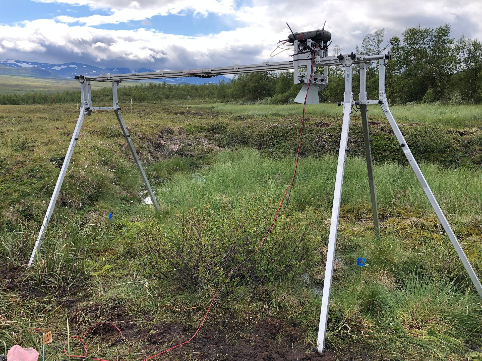
Figure 1. b) Radar-Rig consists of C-band radar, horn antennas, and a motor unit.
The TP method is an analogue to SAR, with the difference of the antennas rotated 90° looking along the track direction. This method allows for vertical backscatter canopy profiles. Both systems have been tested under the TP approach. The UAV-radar system has a high-resolution mapping approximately of 0.5 m along the flight path and 0.5 m vertically (Figure 2), whereas a smaller resolution is achieved with the Radar-Rig (0.22 cm along-track direction, and 3.75 cm vertically, Figure 3).

Figure 2. Tomography profiling image with reconstruction angle of 0° degrees. Path length of 140 m over trees, gaps in the images correspond to a re-setting time of radar. The top figure is co-polarisation (HH) and the bottom is cross-polarisation (VH). Data was collected in the Stoflaket wetland in northeast Sweden.
Although similar platforms exist (Schartel et al. 2018; Charvat, Kempell, and Coleman 2008), the ones developed at the Meteorology Department (University of Reading) are the first of their kind for environmental monitoring applications (e.g. soil moisture, biomass density, etc). The images obtained in a field by these two ground radar systems can be upscaled to interpreted what the satellite imagery are really “seen”. The results will help to understand how the backscatter signal arises spatially and temporally, the issues that can complicate its interpretation and factors that can contribute to signal distortion. This will allow a more complete and timely exploitation of satellite data.
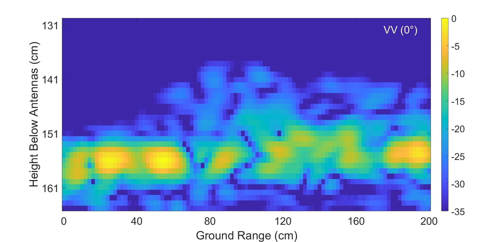
Figure 3. (a) Tomography profiling image with projected angle 0°. Path length of 3m over a dwarf shrub. This top figure (a) is co-polarisation (VV). Data was collected in the Stoflaket wetland in northeast Sweden.

Figure 3. (b) Tomography profiling image with projected angle 0°. Path length of 3m over a dwarf shrub. This bottom figure (b) is cross-polarisation (VH). Data was collected in the Stoflaket wetland in northeast Sweden.
References and Further Reading:
Charvat, Gregory, Leo Kempell, and Chris Coleman. 2008. “A Low-Power High-Sensitivity X-Band Rail SAR Imaging System [Measurement’s Corner].” IEEE Antennas and Propagation Magazine 50 (3):108-15. doi: 10.1109/map.2008.4563576.
Morrison, Keith, and John Bennett. 2014. “Tomographic Profiling—A Technique for Multi-Incidence-Angle Retrieval of the Vertical SAR Backscattering Profiles of Biogeophysical Targets.” IEEE Transactions on Geoscience and Remote Sensing 52 (2):1350-5. doi: 10.1109/tgrs.2013.2250508.
Schartel, Markus, Ralf Burr, Winfried Mayer, Nando Docci, and Christian Waldschmidt. 2018. “UAV-Based Ground Penetrating Synthetic Aperture Radar.” In 2018 IEEE MTT-S International Conference on Microwaves for Intelligent Mobility (ICMIM), 1-4.