
There is much work being done to assess the impact of climate change on the lower atmosphere. Since this is the part of the Earth’s atmosphere affecting the planet’s surface, where (the bulk of!) life on Earth resides, it is imperative that we understand the impact on our biosphere but the higher levels of our atmosphere, that straddle the boundary between Earth and space, are also thought to be affected.

Figure 1: The regions of the Earth’s upper atmosphere. The ionosphere lies within the Thermosphere.
With an increase in CO2 trapping heat in the lower atmosphere, Brasseur and Hitchman (1988) showed that the middle atmosphere is expected to cool. Roble and Dickinson (1989) extended this argument to the upper atmosphere. Assuming a doubling in the concentration of CO2 and methane at 60 km (as then predicted to occur by the mid 21st century), their results indicated that the mesosphere (see figure 1) would be expected to cool by around 5K while the thermosphere (above 200km) would be expected to cool by about 40K. While the thermosphere is difficult to observe directly, a small fraction of the gasses within it are ionised by incoming solar extreme ultraviolet and x-ray radiation to form the ionosphere (figure 2). This electrified region is known to reflect shortwave radio waves (indeed this property enables such signals to be transmitted around the world) and routine observations have been made of the Earth’s ionosphere, most notable at Slough, UK, since 1931 (figure 3).
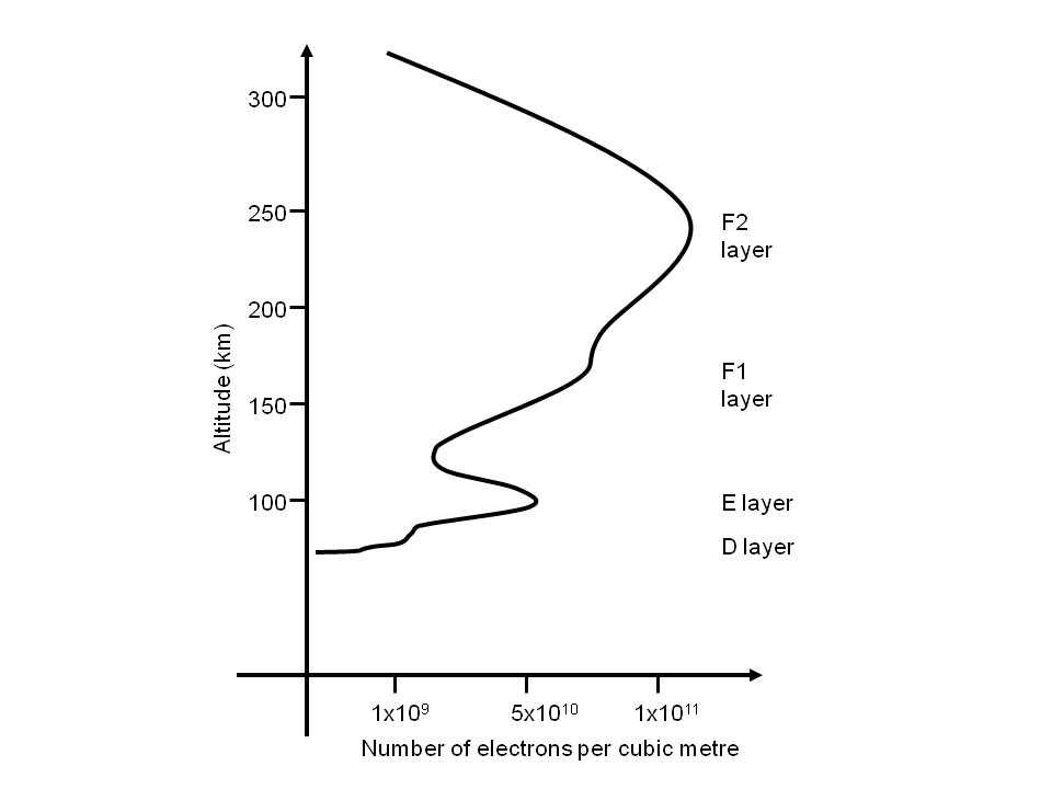
Figure 2: The structure of the Earth’s ionosphere. The upper F-region, in particular, the F2 layer have been the focus for studies into the response of the ionosphere to climate change.
Rishbeth (1990) pointed out that the thermal contraction of the thermosphere is expected to lower the ionospheric F2 layer by 15-20 km, with this estimate being supported by subsequent modelling work (Rishbeth and Roble, 1992). With over ninety years of data now available, this trend should be detectable in the ionospheric records. The first to report on such observations was Bremer (1992) using data from the ionosonde station at Juliusruh in Germany. These data suggested that the height of this layer averaged over seasons, dropped by 8km in 33 years. Subsequently, many others reported observations from different ionospheric stations and the results were far from consistent. Some locations, such as Stanley in the Falkland Islands (Jarvis, 1998), showed a similar decrease, while others, such as Slough in the UK, showed no decrease at all (Bremer, 2004).

Figure 3: Long-term variation in the ionosphere at Slough/Chilton (UK) and Stanley (Falkland Islands). Note the approximately 11 year variation in response to changes in solar x-ray and EUV emissions throughout the solar activity cycle. The peak concentration in each ionospheric layer is expressed in MHz. This radio frequency, (f, Hz), is related to the electron concentration (N, m-3) by the relation f = 8.98√N.
There are several reasons for this apparent disagreement and, as Rishbeth points out in his subsequent article (Rishbeth, 1999), we need to understand the impact of each of these before we have any hope of reliably teasing out a signal due to climate change.
Firstly, while radio measurements of the strength (concentration) of ionisation are very accurate, heights are initially calculated assuming that the radio waves are travelling through free space. A radio wave being reflected from an upper layer has to travel through underlying ionisation and this slows the signal, leading to heights of the upper layers being over-estimated (so-called virtual heights). The influence of this underlying ionisation can be accounted for but any gaps in this information will lead to an uncertainty in the true height of these layers.
Secondly, the ionosphere is created by solar ionisation which is known to vary over an approximately eleven year cycle. While we now have accurate space-based measurements of solar emissions, ionospheric measurements from before the space age require the use of proxies for this radiation, such as the F10.7 index, based on solar radio emissions. In order to be able to remove any bias these indexes need to be carefully calibrated with modern spacecraft observations.

Figure 4: A Coronal Mass Ejection (CME) as imaged by Heliospheric Imager onboard the NASA STEREO mission. The Sun is just outside the frame to the right of the image and the CME is travelling from right to left. The two bright objects are the planets Venus (left) and Mercury (right). Image produced by RAL Space (www.stereo.rl.ac.uk).
Thirdly, solar radiation is only one way that the Sun can affect the Earth’s upper atmosphere. Throughout the solar cycle, vast eruptions of magnetised plasma from the solar atmosphere are ejected through the solar-system (figure 4). If one of these travels past Earth, the magnetic field within the ‘Coronal Mass Ejection’ (CME) can interact with the Earth’s magnetic field, leading to energetic plasma being accelerated into the Earth’s upper atmosphere at the poles, heating the atmosphere there (figure 5). Such heating stirs up the Earth’s atmosphere, causes it to expand and temporarily alters the composition in the upper atmosphere. While some attempts have been made to remove the impact of the heating caused by such events (e.g. Jarvis et al, 1998), the atmospheric composition is more complex to determine, especially in historical records where no direct spacecraft measurements could be made. Scott et al (2014) demonstrated that the annual variability of the ionospheric F-region in long-term records was consistent with changes to the thermospheric composition. A subsequent paper (Scott and Stamper, 2015) showed that these long-term trends varied with location in a way that mapped very closely to the observed trends in ionospheric height (Bremer, 2004), indicating that changes to the chemical composition of the upper atmosphere may be masking any effect due to climate change.
 Figure 5: A schematic showing how energetic particles streaming into the Earth’s atmosphere at the Earth’s polar regions heat the upper atmosphere there, causing it to upwell and subsequently circulate around the globe, temporarily altering the chemical composition of the upper atmosphere.
While it is still possible that a consistent signature of climate change can be extracted from the global ionospheric records, there is much more careful analysis required in order to separate it from the impacts of space weather and global circulation.