By Sadie Bartholomew
Part I: Why
Earth science is a data-driven endeavour. Advanced simulations of the Earth system, whose configurations are themselves complex controlled data, churn out petabytes of analysis datasets whilst raw data from in-situ and satellite observations stream in continuously. Both upstream sources can then undertake a myriad of different paths in processing and post-processing workflows, becoming derived products or being ingested for reanalysis or as a background state to further model runs downstream.
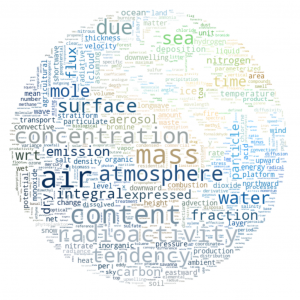
Figure 1: Weather and climate research involves an abundance of data covering many different variables. Individual keywords from potential variables are indicated in this word cloud (optimised to fit the shape and colour of an image of the Earth) generated (for this post) using the Python library word cloud. Read on to learn precisely what terms and weightings are represented!
For the most part this deluge, which epitomises the various “V” words defining “big data”, comes in the form of array-based data packaged into files in a format called netCDF. A major advantage of netCDF is that it was designed to be self-describing, that is to say each file should outline its own structure and each included array of data should be accompanied by a standalone description of what it represents — by metadata.
An underappreciated subclass of data, metadata is indispensable wherever there is a significant collection of information; imagine trying to locate a book in your favourite library if there were no titles, author names or shelf labels.
Involving a mixture of data drawn from the real atmosphere, surface and ocean as well as varying virtual equivalents, geoscience is more complex than a hypothetical library in data terms. Robust, wide-ranging metadata is therefore essential to making sense of it all.
Take the spatio-temporal (space and time) context of the data arrays, for example. Each represents a snapshot of a location on the real or simulated Earth, a sample across one or more of the latitude, longitude, vertical and time coordinates. What is the coverage of the data across these dimensions and how do the arrays map onto them?
Often the correspondence is not simple. To begin with, data frequently covers intervals, or cells, of space-time rather than discrete points on it. In these cases we need to describe the extent of the cells, the so-called bounds, plus the way in which the data in question represents each full cell (perhaps some average or extremum), the cell-methods.
Moreover the data may not be representative of space-time in a straightforward way, potentially spanning a further axis called climatological time in the case of climatological statistics, or by use of a simplified calendar in lieu of the ordinary (Gregorian) calendar. We need a comprehensive and consistent way to describe all these details.
Another core challenge for geoscientific metadata is identifying the nature of the data itself. Assigning a sensible name to a given dataset may not be too taxing, but with such a diversity of potential variables stemming from the wide variety of physical, biogeochemical and human processes at play, doing so unambiguously is really quite difficult.
NetCDF does not standardise the names of data variables, so without further regulation naming would be subject to variance of interpretation across the membership of a diverse research community, sometimes but not always abiding by other named or informal standards from sub-domains that can be at odds. That scenario would add a significant barrier to data sharing, comparison and archival, not only on a human level, but for the other workhorses involved: the machines crunching all that data. Lack of metadata standardisation would cause relevant software packages to become cluttered with logic to handle the countless interpretations and inconsistencies. It would quickly become unmanageable.
Part II: How
So what solution is there? How can we ensure that, now and sustainably going forwards, anyone is able to describe the data encoded in netCDF in a unambiguous way, with scope to fulfil the potential requirements of researchers from multiple disciplines as well as the strict parsing needs of machines?
Step in the CF-netCDF metadata conventions, more commonly known as the CF Conventions.
A community-led effort that spun up shortly after the millennium and has been gaining traction ever since, the CF Conventions set out to solve challenges such as those presented above by providing a definitive standard for climate (‘C’) and forecast (‘F’) metadata. The fundamental scope is to cover netCDF file metadata, though it has been acknowledged that they have wider application and could be used with other data formats, for example XML.
The conventions are outlined in a definitive and comprehensive document that is updated (in the next tagged version) when there is general agreement from interested parties in the community that a proposed change should be made. In this way it has matured over numerous years and versions, with the latest version 1.8 released in February 2020 and 1.9 due out in 2021.
Another core aspect of the conventions is a table establishing a controlled list of possibilities for the names and associated units of data variables. This is the CF Standard Name Table and it is developed in a similar way, though is versioned separately and on version 76 as of late 2020. The idea is that it should provide any name that researchers could conceivably need to describe the data they own or use. If someone can’t find an appropriate name within the table, they submit an Issue on GitHub to formally propose it as a new name and if accepted will form a CF-compliant entity that can be used by all.
Figure 1 in fact depicts all of the individual words taken from the full set of standard names in the current table (the larger the text, the more the given keyword appears throughout the names).
An illustrative indicator of increased uptake of the CF Conventions is the total number of standard names published over time, as shown in Figure 2. To begin with there were around 700 names, now there are nearly 4500 and counting!

Figure 2: The increase in the number of standard names proposed, accepted and finally added into the CF Standard Name Table since the beginning of the project, up to and including version 75, with an indication of the progression of the table versions.
A further indicator is the popularity of annual workshops dedicated to the CF Conventions. 2020’s ‘CF Workshop’ was due to be held in Santander but due to COVID-19 restrictions was held virtually. Over a hundred people registered from fifteen countries, with at least half attending the sessions across each of three days to participate in ways ranging from learning about the current status and future plans of the conventions to engaging in breakout sessions that made headway towards resolving some weighty open proposals. Much interesting discussion took place, all of which is summarised openly on the website, and I, for one, am looking forward to the next annual meeting.
Many colleagues across the department have been involved or indeed instrumental in the growth of the CF Conventions, including Jonathan Gregory who was one of the five original authors and David Hassell who is the present secretary of the Conventions Committee.
Above all, though, the CF Conventions are run and managed by the geoscience community that they serve. Everyone is encouraged to have their say and get involved, be it by commenting to register thoughts on open proposals for changes to the canonical document or for new standard names, raising their own proposals, or helping to develop tools that facilitate discussion or indeed encourage compliance.
If you’re interested in contributing, please explore the official CF Conventions website or dive into the discussions now contained in an Issue Tracker under the official GitHub organisation ‘cf-convention’.


 Figure 1: Annual cycles of rainfall over five East Asian subregions tracked using decomposed moisture fluxes (coloured lines). Sums of each components (solid grey line) are compared to precipitation of ERA-Interim (dotted grey line).