What Is The World Climate Research Programme And Why Do We Need It?

By: Rowan Sutton

My schedule last week was rather awry.  Over four days I took part in a meeting of 50 or so climate scientists from around the world.  Because of the need to span multiple time zones, the session times jumped around, so that on one day we started at 5am and on another day finished at 11pm.  I’m glad I don’t have to do this every week.

But it was a valuable meeting. Specifically, it was a meeting of the Joint Scientific Committee of the World Climate Research Programme, known as WCRP. The WCRP aims to coordinate and focus climate research internationally so that it is as productive and useful as possible. In particular, the WCRP envisions a world “that uses sound, relevant, and timely climate science to ensure a more resilient present and sustainable future for humankind.”

Why does the world need an organisation like WCRP?  The key reason is that climate is both global and local. We humans – approximately 7.96 billion of us at the last count – all live on the same planet.  The global climate can be measured in various ways, but one of the most common and useful measures is the average temperature at the Earth’s surface.  Many factors influence this average temperature and, when it changes significantly, the effects are felt in every corner of the world.  This is what has happened over the last 100 years or so, during which time Earth’s surface temperature has increased by about 1.1oC as a result of rising concentrations of greenhouse gases in the atmosphere.

More specifically, if I want to understand the climate of the UK, I need to consider not only local influences like hills, valleys, forests and fields, but also influences from far away, such as the formation of weather systems over the North Atlantic Ocean. Even climatic events on the other side of the world, such as in the tropical Pacific Ocean, can influence the weather and climate we experience in the UK.

Because climate is both global and local, climate scientists rely heavily on international collaborations.  We need these collaborations to sustain the global network of observations, from both Earth-based and satellite-based platforms, that tell us how climate is changing.  We also rely on international collaborations to share data from the computer simulations that are a key tool for identifying the causes of climate change and for predicting its future evolution.

So now that we are living in a climate emergency, what are the priorities of the World Climate Research Programme? And what were some of the topics at our meeting?  A lot of attention was devoted to questions of priorities: for example, how can we improve our computer simulations as rapidly as possible in directions that will produce the most useful information for policy makers and others? Alongside reducing greenhouse gas emissions, policy makers are increasingly grappling with questions about how societies can adapt to the changes in climate that have already taken place and those that are expected, and how they can become more resilient.  The urgency of these issues is highlighted almost every year now by destructive extreme events we observe around the world – such as the record-shattering heatwave that occurred in Canada last year and the unprecedented flooding in northern Germany and of course we are experiencing a very serious heatwave in the UK right now.

At a personal level, contributing to the WCRP is a privilege.  It brings opportunities to engage with a diverse group of dedicated scientists all working toward very challenging but important shared goals. Through involvement with WCRP over many years I have developed valuable collaborations and made good friends. Whilst COVID has brought many challenges, the growth of online meetings has enabled WCRP to become a more inclusive organisation, which is essential for it to fulfil its mission going forward.  Especially important is the need for two-way sharing of knowledge, ideas and solutions with those working in and with countries in the Global South, which often lack scientific capacity and are particularly vulnerable to the impacts of climate change.  This will be an important focus for a major WCRP Open Science Conference to be held in Rwanda in 2023.

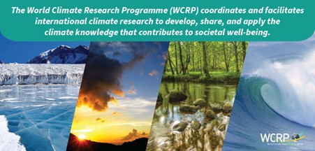
Figure:  More information about the World Climate Research Programme can be found at https://www.wcrp-climate.org/

Posted in Climate change, Climate modelling | Leave a comment

The Golden Age Of Radar

By: Rob Thompson

One of the most frequently viewed pages on weather apps is the radar imagery. We see them on apps, websites and TV forecasts, and have done for years. But rarely do we see much about what we are seeing, and that’s going to change, now.

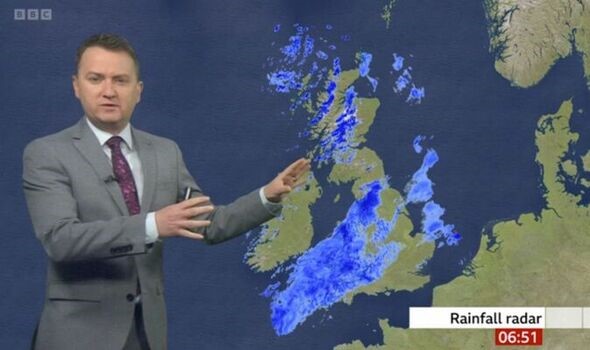
Figure 1: Matt Taylor presenting the radar on the BBC (image source: BBCbreakfast)

The radar maps we see are actually a composite of data taken from 18 different weather radar facilities scattered around the UK and Ireland. The radars are mostly owned by the Environment Agency and MetOffice, operated by the Met Office, though data sharing also gives us data from Jersey Meteorological Department and Met Éireann radars. Each radar is very similar, they send out pulses of microwaves (they have wavelength of 5.6cm) and measure the length of time to get a returned signal from the target precipitation (rain, but also snow, hail, etc. – even flying ants) essentially the same way radar detects aircraft or ships. For the bulk of weather radar’s history, this is what we got, a “reflectivity” which “sees” the rain, and we convert that to a rainfall rate with assumptions on the sizes and numbers of raindrops present (while on the subject of radar and seeing, take a look at the source of the well known “fact” that carrots make you see in the dark). During the 90s and 00s the radars began to also detect the wind from the motion of the drops being detected, which helped, but the data quality remained a problem. It was very difficult to know the source of any power detected, was that power caused by heavy rain? The radar beam hitting the ground? A flock of birds? Or interference? Techniques were used to do our best at finding the power from hydrometeors (rain drops, snow flakes, hail … basically falling water or ice), but they were far from perfect.

But given coverage and software have improved since the first radar was installed in the UK in 1974, why do I think that right now is “the golden age of radar”? The answer is a recent technological leap taken across the UK (and many other worldwide) radars, which was completed in 2019. The new technology uses polarisation (like in glare reducing polarised glasses for driving, fishing etc.) of the microwaves to learn much more information on the particles we are viewing. This means that as well as an overall power of the return, the differences between waves oscillating in the vertical, or horizontal can tell us information on the shape and size of the drops, snow flakes, etc. we view. This means the radars tell us far more about what they are detecting than they did a decade ago, and that means the algorithms for the rainfall maps we see are far better.

Figure 2: New Weather Radar Network infographic  (image source: MetOffice)

We have measurements that detect the shape of the drops – a raindrop is not the tear shape as classically drawn, but small drops (smaller than about 1mm) are spherical, the become more smartie shape as they get larger, falling with the large circle downwards – which tells us how big they are. Some time spent in the front seats of a car will tell you that rain isn’t all the same, sometimes there are a few large drops, other times there are few large drops, but huge numbers of small drops, the radar can now tell the difference. Knowing how real rain, snowflakes, hail but also, birds, insects, aircraft, interference, the sea or the ground appear in the various available radar observations means that the radar network is now able to do a much better job of determining what is a genuine weather signal, and what should be removed – this has hugely reduced the amount of data the network losses and means the network can also detect lighter rainfall. Interference (which causes radar blind spots), has the potential to prevent the radar observing heavy and dangerous rains (such as cause flash flooding), can be traced, which can help prevent it from continuing.

Finally, there’s the actual rainfall rates derived from the radar network. There’s no other way to view a wide area of rainfall on a scale as small as radar can (one kilometer – just over half a mile – squares), and now, with the new radars, the rainfall rate estimates are more accurate than ever before. In the presence of the heaviest rains, with the potential for dangerous flash flooding, the old radars would struggle the most, sometimes failing to see rain at all (see figure 2). The new radar measurements are utilised to improve the rainfall rates, overcoming many of the challenges of the past, helping with a number of potential issues to get accurate rainfall information in near real time.

Figure 3:Heavy rain missed by radar in July 2007.

These are just the things in place now, but there is much more to come and more research to be done. Improvements on detecting the type of precipitation are being developed, corrections to handle the melting of snow (much UK rain falls as snow high above us). New methods of interpreting the data are being considered, and more uses, such as automatic calibration and detection of blocked beams, with more direct use of the radar for initiating weather forecast models being implemented.

It’s a time of huge and rapid improvement for UK weather radar observations and to me, that makes this the golden age of weather radar.

Posted in Climate, earth observation, Flooding, Hydrology, Measurements and instrumentation | Tagged | Leave a comment

Density Surfaces In The Oceans

By: Remi Tailleux

Below the mixed layer, shielded from direct interaction with the atmosphere, ocean fluid parcels are only slowly modified by turbulent mixing processes and become strongly constrained to move along density surfaces of some kind, called `isopycnal’ surfaces. Understanding how best to define and constrain such surfaces is central to the theoretical understanding of the circulation of the ocean and of its water masses and is therefore a key area of research. Because seawater is a complicated fluid with a strongly nonlinear equation of state, the definition of density surfaces has remained ambiguous and controversial. As a result, oceanographers have been using ad-hoc constructs for the past 80 years, none of which are fully satisfactory. Potential density referenced to some constant reference pressure has been one of most widely used of such ad-hoc density constructs. For instance, the variable σ2 denotes the potential density referenced to 2000 dbar. Physically, σrepresents the density (minus 1000 kg/m3) that a parcel would have if displaced from its actual position to the reference pressure 2000 dbar while conserving its heat and salt content. σ0 and σcan be similarly defined for the reference pressure 0 dbar (surface) and 1000 dbar.

Figure 1: Behaviour of different definitions of density surfaces for the 27 degrees West latitude/depth section in the North Atlantic Ocean defined to coincide at about 30 degrees North in the region close to the strait of Gibraltar. The background depicts the Turner angle, whose value indicates how temperature and salinity contribute to the local stratification. The figure illustrates how different definitions of density can be, which is particularly evident north of 40 degrees North. ρref  defines the same surfaces as the variable γTanalytic defined in the text. Also shown are surfaces of constant potential temperature (red line) and constant salinity (grey line).

Potential density, however, is usually assumed to be useful only for the range of pressures close to its reference pressure. As the range of pressures in the ocean varies from 0 dbar to about 11000 dbar (approximately 11,000 meters) in its deepest trenches, it follows that in practice, oceanographers had to resort to using different kind of potential density for different pressure ranges (called patched potential density or PPD). This is not satisfactory, however, because this introduces discontinuities as one moves from one pressure range to the next. To circumvent this difficulty, McDougall (1987) and Jackett and McDougall (1997) introduced a new variable, called empirical neutral density γn, as a continuous analogue of using patched potential density. However, while potential density is a mathematically explicit function that can be manipulated analytically, γn can only be computed by means of a complicated black-box piece of software that only works north of 60N latitude and for the open ocean thus excluding interior seas such as the Mediterranean. The neutral density algorithm works by defining a neutral density surface as made up of all the points that can be connected by a `neutral path’. Two points with pressures p1 and p2 are said to be connected by a neutral path if they have equal values of potential density referenced to the mid pressure (p1+p2)/2. Figure 1 illustrates that different definitions of density can lead to widely different surfaces and therefore how important it is to understand the nature of the problem!

The lack of mathematical expression defining γn, even in principle, has been problematic as it makes it very hard to develop any kind of theoretical analysis of the problem. Recently, we revisited the problem and proposed that γshould be regarded as the approximation of the so-called Lorenz reference density, denoted ρref .  The latter is a special form of potential density, in the sense that it is referenced to a variable reference pressure that physically represents the pressure that a fluid parcel would have in a notional state of rest. This state of rest can be imagined to be the state that the ocean would eventually reach if one were to suddenly turn off the wind forcing, the surface fluxes of heat (due to the sun and exchanges with the atmosphere), and the freshwater fluxes (due to precipitation, evaporation, and river runoff). While this state of rest may sound to be something complicated to compute in practice, Saenz et al. (2015) has developed a clever and efficient way to do it. Figure 2 (a) illustrates an example of such a variable reference pressure field for the 30 degrees West latitude/depth section in the Atlantic Ocean. This shows that in most of the section, the variable reference pressure is close to the actual pressure, which means that over most of the section, fluid parcels are very close to their resting position. This is clearly not the case in the Southern Ocean, however, where reference pressures are in general much larger than their actual pressure. Physically, it means that all fluid parcels in the Southern Ocean `want’ to go near the bottom of the ocean. Tailleux (2016) used this reference pressure to construct a new analytical density variable called γTanalytic that can explain the behaviour of γn almost everywhere in the ocean, as illustrated in Figure 2(b). In contrast to γnγTanalytic has an explicit mathematical expression that can be computed in all parts of the ocean. This is an important result, as it provides for the first time a clear and transparent definition of how to define ‘density surfaces’ in the ocean. Indeed, what this means is that the density surfaces thus defined are simply the density surfaces that would lie flat in a state of rest, which seems the most physically intuitive thing to do, even if this has not been considered before. In contrast, σsurfaces or any other definitions of density surfaces would still exhibit horizontal variations in a resting state, which does not seem right.

Figure 2.: (a) Example of the new variable reference pressure for the latitude/depth section at 30 degrees West in the Atlantic Ocean. (b) Comparison of γn and our new density variable γTanalytic along the same section, demonstrating close agreement almost everywhere except in the Southern Ocean.

An important application is that it now makes it easy to construct `spiciness’ variables,  whose aim is to quantify the property of a fluid parcel of a given density to be either warm and salty (spicy) or cold and fresh (minty). To construct a spiciness variable, simply take any seawater variable (the simplest being salinity and potential temperature), and remove its isopycnal mean. Spiciness is the part of a variable that is advected nearly passively along isopycnal surfaces, where the term `passive’ means being carried by the velocity field without modifying the velocity field. The construction of spiciness variables allows for the study of ocean water masses, as was recently revisited by Tailleux (2021) and illustrated in Figure 3. The construction of γTanalytic  opens many exciting new areas of research, as it promises the possibility of constructing more accurate models of the ocean circulation as will be reported in a future blog!

Figure 3: Different constructions of spiciness using different seawater variables, obtained by removing the isopycnal mean and normalising by the standard deviation, here plotted along the longitude 30W latitude/depth section in the Atlantic Ocean. The blue water mass is called the Antarctic Intermediate Water (AAIW). The Red water mass is the signature of the warm and salty waters from the Mediterranean Sea. The light blue water mass in the Southern Ocean reaching to the bottom is the Antarctic Bottom Water (AABW). The pink water mass flowing in the rest of the Atlantic is the North Atlantic Bottom Water (NABW). The four different spiciness variables shown appear to be approximately independent of the seawater variable chosen to construct them. The variables τ and π used in the top panels are artificial seawater variables constructed to be orthogonal to density in some sense. S and θ and used in the lower panels are salinity and potential temperature.

References

Jackett, D.R., and T.J. McDougal, 1997: A neutral density variable for the world’s ocean. J. Phys. Oceanogr., 27, 237—263. DOI: https://doi.org/10.1175/1520-0485(1997)027%3C0237:ANDVFT%3E2.0.CO;2

McDougall, T.J., 1987: Neutral surfaces. J. Phys. Oceanogr., 17, 1950—1964. DOI: https://doi.org/10.1175/1520-0485(1987)017%3C1950:NS%3E2.0.CO;2

Saenz, J.A., R. Tailleux, E.D. Butler, G.O. Hughes, and K.I.C. Oliver, 2015: Estimating Lorenz’s reference state in an ocean with a nonlinear equation of state for seawater. J. Phys. Oceanogr., 45, 1242—1257. DOI: https://doi.org/10.1175/JPO-D-14-0105.1

Tailleux, R., 2016: Generalized patched potential density and thermodynamic neutral density: Two new physically based quasi-neutral density variables for ocean water masses analyses and circulation studies. J. Phys. Oceanogr., 46, 3571—3584. DOI: https://doi.org/10.1175/JPO-D-16-0072.1

Tailleux, R., 2021: Spiciness theory revisited, with new views on neutral density, orthogonality, and passiveness. Ocean Science, 17, 203—219. DOI: https://doi.org/10.5194/os-17-203-2021


Posted in Climate, Fluid-dynamics, Oceanography, Oceans | Leave a comment

Is Europe At Risk From Hurricanes?

By: Reinhard Schiemann

Growing up in Europe late last century, I would have been a little surprised at this question, and my knee-jerk answer would have been a firm no: hurricanes happened on TV in far-away tropical places, bending and breaking Caribbean palm trees, but not European oaks.

Some thirty years later, I have learnt that this question is worth unpicking a little more. It is true that most North Atlantic hurricanes form over the ocean at low latitudes before travelling west or northwest primarily making landfall over North America’s Gulf and Atlantic coasts where they can cause damage through the strong winds and rain they bring. Some hurricanes do however recurve into an eastward path and eventually reach Europe (Figure 1). They change as they do so, losing the characteristic eye, tending to weaken, and developing warm and cold fronts. In short, some (ex-)hurricanes reach Europe, but they are no longer hurricanes when they do.

Figure 1: Path and lifecycle of Hurricane Katia (August/September 2011).

Recent work at the University of Reading and the National Centre for Atmospheric Science has given us a better idea of how often such storms affect Europe, what properties they have, how damaging they are, and what factors control their incidence. Baker et al. (2020) show that these so-called post-tropical cyclones (PTCs) are rare; about two PTCs make landfall in Europe per year on average with some years seeing none at all and more than five landfalls in other years. Interestingly, in a minority of these storms, aspects of their tropical origin can be recognised even as they make landfall in Europe, and it is these storms that are the windiest PTCs to reach Europe.

Given PTCs are so rare, one might argue that they are a curiosity but not overly important as a source of hazardous weather affecting Europe. To assess their importance fairly, PTCs need to be put in the context of the hundreds of midlatitude storms that affect Europe each year and do not originate in the tropics. This is one of the issues addressed by Elliott Sainsbury, SCENARIO PhD student at the University of Reading. Elliott and his colleagues have shown that, while only about 1% of all storms affecting Europe are PTCs, they constitute about 8% of the systems attaining storm-force winds (Sainsbury et al 2020, Figure 2).

Figure 2: (left) Normalised frequency of post-tropical cyclones (PTCs) and, other, midlatitude cyclones (MLCs) affecting Europe and attaining a given surface windspeed, and (right) the fraction of all storms which are PTCs and attain a given windspeed

In other work, they determined what controls the large variations in the year-to-year number of PTCs (Sainsbury et al. 2022). They show that the number of hurricanes recurving and entering the midlatitude North Atlantic in each year is primarily determined by the total number of hurricanes forming in the tropical Atlantic in the first place. This latter number, also called the activity of the hurricane season, can be predicted with some skill ahead of the season as it is controlled by large-scale and predictable modes of climate variability such as the El Niño Southern Oscillation (ENSO) phenomenon. The results by Sainsbury et al. 2022 are therefore encouraging, as some of the seasonal predictive skill might extend to PTCs affecting midlatitude regions such as Europe.

Finally, it is logical to ask if the number or character of PTCs affecting Europe will change with global warming. The answer is, alas, not known. There is indeed some concern that more of these storms might reach Europe as the North Atlantic Ocean warms (Haarsma et al. 2013), yet climate model simulations do not agree on the future change – Elliott’s ongoing work shows that most models project an end-of-century decrease in the number of North Atlantic hurricanes offset by an increase in the fraction of hurricanes reaching the midlatitudes as PTCs. Crucially, the latest generation of models cannot be trusted to fully capture the physical processes controlling the character and trajectories of hurricanes, and further research and climate model development are needed to address this question with any degree of certainty.

References:

Baker, A. J., K. I. Hodges, R. K. H. Schiemann, and P. L. Vidale, 2021: Historical Variability and Lifecycles of North Atlantic Midlatitude Cyclones Originating in the Tropics. Journal of Geophysical Research: Atmospheres, 126(9), 1–18, https://doi.org/10.1029/2020JD033924.

Haarsma, R. J., W. Hazeleger, C. Severijns, H. de Vries, A. Sterl, R. Bintanja, et al., 2013: More hurricanes to hit western Europe due to global warming. Geophysical Research Letters, 40(9), 1783–1788, https://doi.org/10.1002/grl.50360.

Sainsbury, E. M., R. K. H. Schiemann, K. I. Hodges, L. C. Shaffrey, A. J. Baker, and K. T. Bhatia, 2020: How Important Are Post‐Tropical Cyclones for European Windstorm Risk? Geophysical Research Letters, 47(18), https://doi.org/10.1029/2020GL089853.

Sainsbury, E. M., R. K. H. Schiemann, K. I. Hodges, A. J. Baker, L. C. Shaffrey, and K. T. Bhatia, 2022: What Governs the Interannual Variability of Recurving North Atlantic Tropical Cyclones? Journal of Climate, 35(12), 3627–3641, https://doi.org/10.1175/JCLI-D-21-0712.1.

Posted in Climate, Europe, North Atlantic, Windstorms | Tagged | Leave a comment

Forecasting Rapid Intensification In Hurricanes And Typhoons.

By: Peter Jan Leeuwen

We all know the devastating power of hurricanes, typhoons, and their Southern Hemisphere counterparts. It is crucial that we predict their behaviour accurately to avoid loss of life and to better guide large-scale infrastructure operations. Although tremendous progress has been made, especially in predicting their propagation path, the intensity or wind forecasts are much more difficult. This is related to the fact that the path of a hurricane is largely determined by the large scale atmospheric environment, and we know that environment quite well. However, intensity has to do with small-scale details in the core regions of hurricanes, and these are much harder to predict. The largest unknown is the mysterious rapid intensification, in which the wind speed in a hurricane can increase from 50 km/h to an astonishing 300 km/h in two days.

Figure 1: a) Satellite view of Hurricane Patricia just before landfall, and b) maximum wind at 10 m above the sea surface in Hurricane Patricia (Note 1 m/s corresponds to 3.6 km/h).

 Hurricane Patricia (see figures 1a and b)  in 2015 holds the rapid-intensification record and we have studied her in detail. Fortunately, we had an exceptionally detailed data set of temperature, humidity and wind fields in the inner region of the Hurricane from aircraft measurements. (Indeed, they did fly the plane straight through the core of the Hurricane…)  This provided an unprecedented view of the inner structure of the Hurricane, but also allows us to study the influence of these observations on prediction.

For this prediction we update the model fields, such as the temperature field and the wind field, using a technique called data assimilation. Data assimilation is a systematic method to incorporate observations into computer models (see e.g. the open access book Evensen et al, 2022, with over 40,000 downloads). For the results below we use a state-of-the-art Local Ensemble Transform Ensemble Kalman Filter, abbreviated to LETKF (see Tao et al. 2022 for details of this study). We run two experiments, one in which we assimilated only large-scale satellite data, and one in which we added the aircraft data of the inner hurricane regions. This resulted in two forecast ensembles, the yellow-brown lines and the blue lines in figure 2.

Figure 2: The strength of the wind as function of distance to the centre of the Hurricane.  Data from two forecast ensembles, one ensemble based on only satellite data (yellow-brown) and one ensemble based on both the satellite and the aircraft data (blue). The purple lines are not important here. Note that the aircraft data give rise to much higher velocities because they resolve much smaller scales.

Figure 2 shows that the ensemble based on the aircraft data (blue lines) shows much higher wind speeds, and these hurricanes all develop a rapid intensification phase and become major category 5 hurricanes. The yellow-brown lines do not use the aircraft data, have much lower wind speeds, and do not develop into strong hurricanes. We conclude that the detailed data in the inner part of the Hurricane are crucial for a proper prediction of the intensity of Hurricanes.

These model predictions can be studied further using techniques from causal discovery developed for Hurricane dynamics (Van Leeuwen et al. 2021). Causal discovery methods try to find cause and effect relations in hurricane evolution. The weaker Hurricanes that do not develop rapid intensification have different connections between the temperature and the wind fields than those hurricanes that do show rapid intensification. Specifically, what is needed for rapid intensification is a collaborative action of the temperature and humidity at the sea surface, strong upward motion in the core region, and rain and snow formation in the region close to the centre of the Hurricane, as well as strong heating of the centre region from the stratosphere. All these work together to heat up the core region of the Hurricane, which provides the energy to increase the winds. These winds bring in more humidity near the sea surface, leading to more rain and snow formation, leading to further heating etc. If all these processes work in Harmony rapid intensification is the result. In contrast, when one of these processes is out of sink, as with the yellow-brown lines, the Hurricane does not grow fast and rapid intensification does not occur.

Concluding, although our understanding keeps increasing there are still many missing parts. One way forward is to use better ways to bring the observations into the prediction models. The methods used today, such as the LETKF mentioned above, are based on linearizations that do not allow us to extract all relevant information from the data. This can lead to incorrect interpretation of the causal relations between hurricane variables. New fully nonlinear data-assimilation methods have been developed (e.g. Hu and Van Leeuwen, 2021) and we are working on implementing these in Hurricane prediction models to improve predictions and to understand these major ‘freaks of nature’ better.

References:

Evensen, G., F.M. Vossepoel, and P.J. van Leeuwen (2022) Data Assimilation Fundamentals, Springer, doi: 10.1007/978-3-030-96709-3  (free to download)

Hu, C-C, and P.J. van Leeuwen (2021) A particle flow filter for fully nonlinear high-dimensional data assimilation., Q.J. Royal Meteorol. Soc.,  doi:10.1002/qj.4028

Tao, D., van Leeuwen, P. J., Bell, M., and Ying, Y. (2022). Dynamics and predictability of tropical cyclone rapid intensification in ensemble simulations of Hurricane Patricia (2015). Journal of Geophysical Research: Atmospheres, 127, doi:10.1029/2021JD036079

Van Leeuwen, P.J., M. DeCaria, N. Chakraborty, and M. Pulido (2021) A new framework for causal discovery, Chaos, 31, 123128, doi:10.1063/5.0054228

Posted in Climate, Predictability, Tropical cyclones | Tagged | Leave a comment

A Different Kind Of Turbulence

By Miguel Teixeira

It might be thought that turbulence is essentially the same everywhere. However, its mixing efficiency depends not only on its intensity (as might be expected intuitively), but also on more subtle properties, such as its anisotropy (which components of the velocity fluctuations are dominant). These characteristics are determined by the mechanisms that generate the turbulence. For example, it is known that convective turbulence (generated by positive heat fluxes into the atmosphere or negative heat fluxes out of the ocean) typically mixes more efficiently than shear-generated turbulence induced by the no-slip boundary condition at the ground. This is not only because heating is often a more potent source of energy than wind shear, but also because convective turbulence is dominated by its vertical velocity fluctuations (which have a greater mixing ability – in the vertical), whereas shear turbulence is dominated by horizontal velocity fluctuations.

Even ignoring thermal effects, turbulence in the oceanic boundary layer has a totally different character from that of atmospheric boundary layer turbulence, because of the different boundary conditions at the air-water interface relative to those at the ground. While, in the atmosphere over flat terrain (undulating terrain is different), the no-slip boundary condition generates shear-driven turbulence, in the oceanic boundary layer, a sheared water current exists near the surface, forced by the wind stress, but it is not the most important aspect. The wind stress also generates surface waves, which have an associated Lagrangian transport in the direction of wave propagation, named “Stokes drift”. This element totally changes the character of the turbulence.

Figure 1 shows foam alignments at the surface of a body of water. This foam, which was probably produced by micro-breaking or white-capping of the surface waves (also caused by the wind), is aligned perpendicularly to the crests of the waves (at least far from the shore) and is also roughly aligned with the wind. This happens because of the presence of coherent vortices (known as Langmuir circulations) in the water, with their axes aligned with both the wind and wave propagation direction. The foam collects at the convergence zones of these vortices at the air-water interface.

Figure 1: Windrows, or foam alignments at the air-water interface of a body of water, induced by the joint effects of a surface current induced by the wind and surface waves via Langmuir Circulations.

Although Langmuir circulations were initially studied as single-scale features, using modal growth linear theories (Craik and Leibovich, 1976), it has become clear that they have multiple scales, so they can be viewed as a separate type of turbulence (named Langmuir turbulence) (McWilliams et al., 1997), distinct from the shear-driven turbulence more common in non-convective boundary layers. The general configuration of Langmuir turbulence is described in Figure 2. The streamwise vortices that dominate Langmuir turbulence are typically aligned with the direction of propagation of surface waves, and within 5˚ to 15˚ of the wind direction. They are characterized by convergence zones (in blue) where foam (or floating debris) collects, vertical velocities of ~5 u*, where u* is the friction velocity in the water, and surface jets at the convergence zones in the direction of both the wind and waves, with velocity perturbations of ~10 – 15 u*. The upwelling/surface-divergence zones of Langmuir vortices are privileged locations for the emergence of plankton.

Figure 2: Schematic diagram showing the configuration of Langmuir turbulence vortices and the associated physical phenomena (from Smith, 2001).

The mechanisms underlying the structure of Langmuir turbulence, and its differences from shear turbulence, are explained in Figure 3. On the left panel, we can see how vertical vorticity (which always exists in turbulence) is tilted and stretched by the vertical profile of the Stokes drift associated with surface waves propagating from left to right. This Lagrangian transport has a maximum at the surface and decays to zero as depth increases. This causes a tilting of the vertical vorticity into the direction of the Stokes drift (which coincides with the direction of wave propagation), and stretching of this vorticity. We will call the wave propagation direction, which typically coincides with the direction of the wind stress and of the shear in the current induced by the wind, the streamwise direction. Stretching of the streamwise vorticity causes its amplification, making this vorticity become dominant in the turbulence. This explains the existence of coherent streamwise vortices in Langmuir turbulence. These vortices are dominated by velocity fluctuations in the spanwise and vertical directions, the latter strongly promoting vertical mixing.

On the right panel of Figure 3, we see how shear-driven turbulence differs from Langmuir turbulence in this respect. Vertical vorticity in the turbulence is equally tilted and stretched into the streamwise direction, now by mean shear in the wind-driven current. But the mean vorticity in the current is also tilted by the circulation induced by the turbulent vorticity, and this causes a partial cancellation of the latter. This is why shear-driven turbulence is not dominated by streamwise vortices, like Langmuir turbulence. Rather, velocity fluctuations in the streamwise direction (sometimes called “streaky structures”) are dominant.

Figure 3: Left: tilting and stretching of vertical vorticity into streamwise vorticity by the Stokes drift of surface waves; Right: tilting and stretching of vorticity in a shear flow (from Teixeira and Belcher, 2002).

The consequences of these differences for the transport of buoyant tracers trapped at the air-water interface are explained in Figure 4 (where a surface wave is assumed to propagate from left to right and/or a wind is assumed to blow from left to right). In wave-driven (or Langmuir) turbulence (diagram on the left), the flow is dominated by streamwise vortices, which at the surface induce primarily spanwise velocity fluctuations (arrows). The convergence zones of this velocity field lead to the concentration of buoyant tracers along lines aligned in the streamwise direction. In shear-driven turbulence (diagram on the right), there is also a tendency for buoyant surface tracers to align in the streamwise direction, but the mechanism that causes it is weaker. This is associated with the confluence that necessarily occurs at the entrance regions to maxima in the dominant streamwise velocity fluctuations (streaky structures).

Figure 4: Schematic diagrams showing the transport of buoyant tracers by (Left) streamwise vortices in Langmuir turbulence; (Right) streaky structures in shear-driven turbulence (from Teixeira and Belcher, 2010).

An up-to-date overview of Langmuir turbulence, including motivation of its importance, recent developments in theory, measurements and numerical modelling, and various applications, is provided in a recent short review by the author of this post , published in the latest edition of the Encyclopedia of Ocean Sciences (Teixeira, 2019).

References

Craik, A. D. D., and Leibovich, S. (1976) A rational model for Langmuir circulations. J. Fluid Mech., 73, 401-426. doi: https://doi.org/10.1017/S0022112076001420

McWilliams, J. C., Sullivan, P. P. and Moeng, C.-H. (1997) Langmuir turbulence in the ocean. J. Fluid Mech., 334, 1-30. doi: https://doi.org/10.1017/S0022112096004375

Smith, J. A. (2001) Observations and theories of Langmuir circulation: a story of mixing. In Fluid Dynamics and the Environment: Dynamical Approaches, Lecture Notes in Physics, vol. 566, 295-314, Ed.: Lumley, J.L., Springer. doi: https://doi.org/10.1007/3-540-44512-9_16

Teixeira, M. A. C. (2019) Langmuir circulation and instability. In Encyclopedia of Ocean Sciences (Third Edition), Eds. J. K. Cochran, H. J. Bokuniewicz, P. L. Yager, Academic Press, pp. 92-106. doi: https://doi.org/10.1016/B978-0-12-409548-9.04176-2

Teixeira, M. A. C. and Belcher, S. E. (2002) On the distortion of turbulence by a progressive surface wave. J. Fluid Mech., 458, 229-267. doi: https://doi.org/10.1017/S0022112002007838

Teixeira, M. A. C. and Belcher, S. E. (2010) On the structure of Langmuir turbulence. Ocean Modelling, 31, 105-119. doi: https://doi.org/10.1016/j.ocemod.2009.10.007


Posted in Boundary layer, Climate, Environmental physics, Fluid-dynamics, Oceans, Turbulence, Waves | Leave a comment

What are the challenges in forecasting the impacts of tropical cyclones?

By: Liz Stephens

Last year I joined the Meteorology department in a joint-post between the University of Reading and the Red Cross Red Crescent Climate Centre (RCCC), but I still suspect most people have no idea exactly what it is that I do! Apart from the administrative team in the Netherlands, the Climate Centre is virtual, we have 40+ team members based all around the world which makes for a wonderful blend of cultures (and a sometimes confusing use of humour and local proverbs!).

My role is as the Science Lead for Anticipatory Action, which means I help steer efforts to use forecasts to take actions to support vulnerable communities in advance of a disaster. We develop so-called Early Action Protocols (EAPs, plans to secure pre-agreed financing in advance of a disaster) for taking actions before different types of hazard. These EAPs are required to show evidence of forecast skill, which is often a challenge where forecast archives or observational data is limited.

This work aligns very well with the research I have been leading under the Science for Humanitarian Emergencies and Resilience research programme. We have supported the assessment of flood forecast skill in Uganda, which has informed where in the country Anticipatory Action is feasible. We have also produced flood forecast bulletins for the Foreign Commonwealth and Development Office (FCDO), firstly, for Tropical Cyclone Idai in 2019, but then with continued funding to produce these for many tropical cyclones with associated flood impacts in vulnerable countries.

Figure 1: Mocuba District in Nampula Province. (c) Mozambique Red Cross Society

The intersection between my two roles has been even more apparent in the last year. Super typhoon Rai (Odette) in the Philippines caused enormous impacts just before Christmas in 2021, but due to rapid intensification the forecasts of the storm had limited accuracy beyond 12 hours before landfall; nowhere near enough time to trigger the release of financing. I spoke about this more on “Science in Action” for the BBC World Service (https://www.bbc.co.uk/sounds/play/w3ct1l4s, from 9 minutes in). I was invited to join a panel discussion at a workshop led by the Start Network in January to discuss how to address the challenges that rapid intensification gives us within our decision-making, commenting on research presented by the University of Philippines and PAGASA on rapid intensification. (The Reading link continues, with PhD researcher BA Racoma also joining the workshop, and with one of the presenters having Ed Hawkins’s climate stripes in the background).

Earlier this year we saw the devastating impact of a series of tropical cyclones in the Southern Indian Ocean (Ana, Batsirai, Emnati, Gombe), affecting Madagascar, Mozambique and Malawi. Along with the wider team of scientists from ECMWF, University of Bristol and HR Wallingford, we (University of Reading) produced flood forecast bulletins for FCDO to provide onto humanitarian partners. These bulletins provide support to humanitarians operating on the ground, and inform the release of funds by the government to support these operations (e.g. https://www.gov.uk/government/news/uk-provides-emergency-support-to-madagascar-after-cyclone-batsirai). With colleagues at RCCC we provided early awareness to the National Red Cross Societies that we support of the potential for impacts, providing interpretation of the forecast uncertainties and likely areas worse hit.

Figure 2: Global Flood Awareness System (GloFAS) forecasts for Tropical Cyclone Batsirai, February 2022. Colour saturation represents the probability of a 1 in 5 year return period flood.

The learning across all of these cyclones is that for early warning and humanitarian decision-making there is a massive need to improve the provision of multi-hazard early warnings – too often the forecast information coming in is fragmented, with one source for wind, another for river floods, another for storm-surge flooding and so on. To make robust decisions we need to combine the hazard forecasts to provide comprehensive assessments of exposure and vulnerability, giving us an overall assessment of risk that will help to prioritise resources, determine early actions and provide appropriate impact-based warnings. This of course needs to be led by the national meteorological, hydrological and disaster management authorities.

Posted in Climate, Flooding, Tropical cyclones, Weather forecasting | Leave a comment

Co-Producing New Sub-Seasonal Weather Forecasts in Africa

By: Linda Hirons

Weather-related extremes affect the lives and livelihoods of millions of people across tropical Africa. Access to reliable, actionable weather information is key to improving the resilience of African populations and economies. Specifically, at the extended sub-seasonal timescale (forecasts of 1-4 weeks ahead), improved weather information could be transformational in building better early warning systems for the extreme events which cause infrastructural and societal damage. However, the uptake and availability of accurate weather information and services on these extended timescales remain very low across the continent.

Recent scientific advances have improved our understanding of what drives changes in weather on these timescales (e.g., the Madden Julian Oscillation (MJO); Zaitchik 2017) and subsequent modelling advances have enabled us to better represent these drivers (e.g., Vitart et al 2017) and their local impacts across Africa (e.g., de Andrade et al 2021). While these scientific and modelling advances are necessary to improve forecasts it is becoming increasingly clear that they are not sufficient to translate advances in knowledge into real tangible societal benefits. This requires a more collaborative and iterative approach where knowledge from scientists is combined with knowledge from local forecasters and knowledge from the specific decision-making context of forecast users to jointly co-produce (e.g., Vincent et al 2018) bespoke weather and climate services which can be truly effective.

Figure 1: The building blocks (a) and principles of good co-production (b) introduced in Carter et al. (2019) 

Through a Real-Time Pilot Initiative of the WMO Sub-seasonal to Seasonal Prediction Project, the GCRF African-SWIFT and ForPAc projects ran a two-year, sub-seasonal forecasting testbed (Hirons et al 2021) – a forum where prototype forecast products were co-produced and operationally trialled in real-time. Launched in November 2019 in Kenya, the testbed brought together national meteorological services, universities and forecast users from across tropical Africa, to use a co-production approach (Figure 1; Carter et al 2019) to improve the appropriate use of sub-seasonal forecasts. This testbed made real-time, sub-seasonal forecast data from the European Centre for Medium-Range Weather Forecasts (ECMWF) available to users in a range of sectors, including energy, health, agriculture, disaster risk reduction and food security across tropical Africa.

The sub-seasonal testbed has been providing co-produced, tailored forecast products and advisories to weather-sensitive sectors across Africa (Hirons et al 2021). Examples here from users in the energy sector in Kenya and the health sector across the Sahel exemplify the local application and benefits of new testbed forecast products.

In Kenya, sub-seasonal forecasts co-produced by the Kenya Meteorological Department and the Kenya Electricity Generating Company (KenGEN), which is responsible for supplying more than 70% of Kenya’s electricity, supported improved hydropower planning. Hydropower accounts for approximately 45% of KenGEN’s total supply and fills the gaps when other sources like solar or wind are unreliable. It uses fast-moving water to produce electricity so Kenya relies on key dams for sufficient water storage. Previously dam levels would have been systematically lowered before the start of the rainy season in anticipation of significant rainfall. However, if rains failed, drought could cause considerable interruptions to the power supply and increase reliance on diesel generators. Through the Testbed KenGEN has been incorporating the sub-seasonal rainfall information into their dam management decisions enabling them to maximise dam levels without overflowing and causing downstream flooding. During the Testbed Kenya has experienced uninterrupted power, even through periods of drought, and has eliminated emergency diesel generators from the national electricity grid entirely.

Figure 2: Example of the vigilance map for the emergence of meningitis outbreaks in Africa co-produced with GCRF African SWIFT project and WHO.

Across the Sahel GCRF African SWIFT researchers and forecast producers have been working closely with the World Health Organisation (WHO) to supply bespoke, multi-variable sub-seasonal forecast information for meningitis vigilance across 26 countries in the meningitis belt. It is well known that meningitis outbreaks are more likely in warm, dry conditions, particularly after dust events. Previously the observed environmental conditions were used to determine the likelihood of outbreaks. However, by combining forecasts of temperature, relative humidity and wind speed and direction with dust forecasts, the sub-seasonal testbed has extended the lead time of the existing vigilance maps by up to 2 weeks (Figure 2). Working closely with the WHO has shown that this information has huge implications for improving preparedness action and making timely life-saving interventions to prevent outbreaks.

The GCRF African SWIFT sub-seasonal testbed is coming to an end this year and the focus will be on ensuring that the knowledge co-produced through these collaborative partnerships can be institutionalised and become part of in-country standard operational procedure to ensure project-initiated services are sustained. However, continuing to provide these new services requires national meteorological agencies in Africa to continue to have access to sub-seasonal data in real-time. Surely these direct and tangible societal benefits are enough to convince data providers?

References

Carter, S., Steynor, A., Waagsaether, K., Vincent, K., Visman, E., 2019. Co-production of African weather and climate services. Manual, Cape Town: SouthSouthNorth. https://futureclimateafrica.org/coproduction-manual.

de Andrade, F. M., Young, M. P., MacLeod, D., Hirons, L. C.Woolnough, S. J. and Black, E. (2021) Subseasonal precipitation prediction for Africa: forecast evaluation and sources of predictability. Weather and Forecasting, 36 (1). pp. 265-284. ISSN 0882-8156 doi: https://doi.org/10.1175/WAF-D-20-0054.1

Hirons L., Thompson, E., Dione, C., Indasi, V.S., et al. Using co-production to improve the appropriate use of sub-seasonal forecasts in Africa. Climate Services, 23. 100246. ISSN 2405-8807 (2021)   https://doi.org/10.1016/j.cliser.2021.100246

Vincent, K., Daly, M., Scannell, C., Leathes, B., 2018. What can climate services learn from theory and practice of co-production? Climate Services. 12, 48-58.

Vitart, F., Ardilouze, C., Bonet, A., Brookshaw, A., Chen, M., Codorean, C.,  2017. The sub‐seasonal to seasonal prediction (S2S) project database. Bull. Am. Meteorol. Soc. 98, 163–173

Zaitchik, B.F., 2017. Madden-Jullian Oscillation impacts on tropical African precipitation. Atmospheric Research.184, 88-102.

Posted in Climate, Co-production, Energy meteorology, Forecasting Testbed, Madden-Julian Oscillation (MJO), Predictability, Renewable energy, Seasonal forecasting, subseasonal forecasting, Tropical convection, Weather forecasting | Tagged , , | Leave a comment

Are There Climate Consequences of Using Hydrogen as a Replacement for Coal, Gas and Oil?

By: Keith Shine

There are many possible avenues to reduce carbon dioxide emissions. One of these is a shift to using hydrogen (H2) as a fuel source; it could potentially be used for many current CO2-emitting activities, including industry, heating in the home and transport. There would be many challenges, but it is widely regarded as one component of pathways to reach “net zero”, which aims to stabilise human-induced climate change. A recent Royal Society briefing provides much information on the technological and economic challenges of a move to a hydrogen economy.

As with all potential climate-change solutions, it is necessary to assess their environmental impact. I played a small role in a modelling study on the “Atmospheric Implications of Increased Hydrogen Use”, led by the University of Cambridge (Warwick et al., 2022), funded by the Government’s Department for Business, Energy & Industrial Strategy. Studies of hydrogen’s climate impact go back about 20 years (e.g., Derwent et al. 2006; Schulz et al. 2003; Warwick et al.  2004) but there is now more urgency in understanding the issues (e.g., Derwent et al., 2020; Paulot et al., 2021).

The first issue is how hydrogen is generated. The “feedstock” is simply water. But it takes energy to split hydrogen from water, and it matters where that energy comes from.  There are two low carbon methods. So-called “blue hydrogen” is generated using fossil fuels, but the CO2 produced is captured and stored rather than emitted into the atmosphere.  “Green hydrogen” is generated using renewable energy sources. My focus is the impact of any hydrogen leakage during production, storage and distribution (e.g., from pipework and valves). (The use of the hydrogen just leads to the generation of water.)

Hydrogen itself is of little direct concern, from a climate point of view, although it can impact air quality; the Cambridge study focused on hydrogen’s role in altering the chemistry of the atmosphere, thereby changing concentrations of gases that can influence climate.

A major route to climate impact is via changes in concentrations of a very reactive molecule, the hydroxyl radical (OH), a gas present in tiny quantities but which plays a key role in atmospheric chemistry. It is sometimes referred to as an “atmospheric detergent” as it hastens the removal of many atmospheric pollutants. Leakage of hydrogen reduces OH concentrations, so reducing this cleansing capacity.

The effects of both the hydrogen itself and its impact on OH include increased concentrations of methane, tropospheric ozone and stratospheric water vapour; all these lead to climate warming. It is important to quantify these impacts, and identify uncertainties, to be clear that the climate advantages of reduced CO2 emissions far outweigh the impacts of increased hydrogen use.

My involvement in the Cambridge study was to help quantify the 100-year Global Warming Potential (GWP(100)), a metric to characterise the climate impact of emissions of a gas (relative to the emission of an equal mass of carbon dioxide). GWP(100) is just one possible metric to quantify climate impacts of emissions and in itself is quite contentious: see this blog post by my colleague Bill Collins. But contentious or not, it is widely used in policy applications, including national and international policy agreements.

Warwick et al. (2022) concluded that hydrogen’s GWP(100) was 11±5; about half came from its impact on methane and about a quarter each came from its impact on tropospheric ozone and stratospheric water vapour (some of which was due to a knock-on effect of methane changes).  Clearly uncertainties are substantial, one of which is the atmospheric lifetime of hydrogen which is believed to be 2 to 3 years. As noted above, it is removed by reaction with OH but it is also removed by reactions with soil; the strength of this “soil sink” is particularly uncertain.

So hydrogen leakage does have a higher climate impact (as measured by GWP(100)) than CO2 per kg emitted.  However, hydrogen emissions would be much smaller than the CO2 emissions that they would replace. For one illustrative future scenario, Warwick et al. (2022) estimate that hydrogen’s climate impact would be around 0.4 to 4% (for hydrogen leakage rates of 1 to 10% respectively) of the avoided “CO2-equivalent” emissions. This is all promising but nevertheless there can be no complacency. Leakage rates must be minimised. Remaining uncertainties in quantifying the climate impact must be reduced. The Natural Environment Research Council recently announced a funding opportunity “Environmental response to hydrogen emissions” to help reduce uncertainties.

Electric Car: BMW I Hydrogen Fuel Cell version of the X5 SUV (photo Marco Verch, Creative Commons 2.0)

References:

Derwent, R., P. Simmonds, P., S. O’Doherty, A. Manning, W. Collins, and D. Stevenson, D 2006: Global environmental impacts of the hydrogen economy. International Journal of Nuclear Hydrogen Production and Applications, 1, 57-67 10.1504/IJNHPA.2006.009869

Derwent, R. G., D. S. Stevenson, S. R. Utembe, M. E. Jenkin, A. H. Khan, and D. E. Shallcross, 2020: Global modelling studies of hydrogen and its isotopomers using STOCHEM-CRI: Likely radiative forcing consequences of a future hydrogen economy. International Journal of Hydrogen Energy, 45, 9211-9221. 10.1016/j.ijhydene.2020.01.125

Paulot, F., D. Paynter, V. Naik, S. Malyshev, R. Menzel, and L. W. Horowitz, 2021: Global modeling of hydrogen using GFDL-AM4.1: Sensitivity of soil removal and radiative forcing. International Journal of Hydrogen Energy, 46, 13446-13460. 10.1016/j.ijhydene.2021.01.088

Schulz, M.G., T. Diehl, G.P. Brasseur, and W. Zittel, 2003: Air Pollution and Climate-Forcing Impacts of a Global Hydrogen Economy. Science, 302, 624-627, DOI: 10.1126/science.1089527

Warwick, N. J., S. Bekki, E. G. Nisbet, and J. A. Pyle, 2004: Impact of a hydrogen economy on the stratosphere and troposphere studied in a 2-D model. Geophysical Research Letters, 31. 10.1029/2003gl019224

Warwick, N., P. Griffiths. J. Keeble, A. Archibald, J. Pyle and K. Shine, 2022 Atmospheric implications of increased hydrogen use. Department for Business, Energy & Industrial Strategy Policy Paper https://www.gov.uk/government/publications/atmospheric-implications-of-increased-hydrogen-use

Posted in Atmospheric chemistry, Climate, Climate change, Greenhouse gases, Renewable energy | Leave a comment

Fieldwork Without The Footprint

By: Joy Singarayer

Over the past two years, we have all faced challenges to our working patterns due to the Covid-19 pandemic. Researchers undertaking overseas fieldwork have found many ways to redefine, reschedule, and adapt their approaches in light of travel restrictions (Forrester, 2020). My colleagues and I faced similar challenges when we began a project in the very first month of the first UK lockdown of 2020. While there have been many issues, there have also been opportunities for us to begin to reflect on our responsibilities to communities and individuals involved in field research, and to the carbon footprint of the project.

Until recently, I had not really given a lot of thought to how the data I was using to compare to climate model simulations was extracted, who was involved, or whether they were appropriately acknowledged. My research has focussed on past (prehistoric) climate change, primarily in the tropics, and the data I was using has been processed from the mud at the bottom of lakes or the stalactites from caves taken from around the world by many other scientists over decades. However, a recent decision to venture into new research avenues led to a collaboration with Prof. Nick Branch (SAGES) and scientists from the UK and South America, which has fieldwork as a central part of the project.

The aim of the research is to examine the impacts of current and future climate change on water supplying ecosystems for agriculture in the Peruvian Andes. Our project is called CROPP (Climate Resilience and fOod Production in Peru) and is funded by the Royal Academy of Engineering. It brings together an international and multidisciplinary team of social scientists, hydrologists, ecologists, climatologists, and NGOs to understand the Andean water systems and their contribution to resilience in the face of climate change. This means working directly with remote farming communities and a large funding commitment in the fieldwork budget for the UK team to undertake annual trips to Peru.

Figure 1: An example, from one of our study areas, of the varied landscape in the Ancash region of Peru – Glacial mountain peak (Huascarán), agricultural fields, and ancient human-made water courses.

The initial excitement at the prospect of working across subject boundaries and continents turned to uncertainty about when travel would be allowed and what alternative approaches could be taken to progress the research. The collection and synthesis of secondary data was an obvious way to begin while we waited to see the full extent of the impact of covid. Several months and numerous international video meetings later, we knew that it would be the South American team undertaking the first fieldwork without direct UK input.

Through our partners in Peru, we have employed local research coordinators to engage with farmers (once safe to do so) to produce and collate agro-economic and social science information through conversations and diaries. During the field season last year, we were also able to hire local student research assistants to work with the South American team to conduct hydrological and ecological field research, with remote support from the UK hydrologists. The researchers have produced excellent new data and the approach has worked well. Significant modifications to the budgets were required but our funder has been incredibly helpful in allowing us the flexibility to do this. As a result, we are thankfully in a decent position at the end of the second year of the project, although there is a lot more to do before we can pull the results together. There are also some aspects of the fieldwork that the UK team will need to undertake in person this year.

That said, we have so far saved 15-20 tonnes CO2 (depending on the emissions calculator used) by reducing our international travel, which is roughly equivalent to the annual emissions of between one and two average UK individuals or between eight to eleven average individuals in Peru (note – these figures vary depending on whether you include imports/exports or just territorial emissions). This feels like a positive outcome that we would want to repeat in future projects. In some ways, the new fieldwork set up may also allow more effective community engagement via trusted local research coordinators.

However, there is much more for us to consider in terms of using this opportunity to set up ethical field research practices that address inequalities and the often extractivist nature of field research in the global south, whereby field data are taken and processed in the global north to create outputs without co-development or proper attribution (Bates, 2020; Dunia et al., 2020; Sukarieh and Tannock, 2019). This is particularly so if we are to continue to reduce international travel and undertake more remote field research involving research assistants in other countries. Dunia et al (2020), for example, outline ways to begin to approach this, from rethinking how we view co-authorship so that we include those facilitating research in remote settings, to proper compensation and insurance. There are also broader responsibilities beyond those directly undertaking field research. For example, funding agencies could request details about how the research field practice will be fair and transparent for all involved, and journal reviewers and editors should flag questions about this aspect of the research when manuscripts are submitted.

The changes we initially made to our field research were due to travel restrictions forced on us by covid, but are now undertaking a different journey exploring our responsibilities to construct fair, sustainable, and creative ways of working.

References:

Bates, J, 2020. Reimagining fieldwork during and beyond the pandemic. Feminist Perspectives blog, Kings College London. At: https://www.kcl.ac.uk/reimagining-fieldwork-during-and-beyond-the-pandemic

Dunia O. A., Eriksson Baaz M.,  Mwambari D., Parashar S., Toppo A.O.M. and Vincent J.B.M, 2020. The Covid-19 Opportunity: Creating More Ethical and Sustainable Research Practices. Items: insights from the Social Sciences. At: https://items.ssrc.org/covid-19-and-the-social-sciences/social-research-and-insecurity/the-covid-19-opportunity-creating-more-ethical-and-sustainable-research-practices/

Forrester, N., 2020. How to manage when your fieldwork is cancelled. Nature, Career Feature: doi: https://doi.org/10.1038/d41586-020-03368-0

 Sukarieh M. and Tannock S., 2019. Subcontracting Academia: Alienation, Exploitation and Disillusionment in the UK Overseas Syrian Refugee Research Industry. Antipode: a radical journal of geography, 51(2), 664-680. https://doi.org/10.1111/anti.12502

Posted in Climate, Climate change, Covid-19, Data collection, Diversity and Inclusion, Fieldwork | Leave a comment